Computes Moran's I, a measure of spatial autocorrelation that tests whether values are more similar (positive autocorrelation) or dissimilar (negative autocorrelation) among spatial neighbors than expected by chance.
Arguments
- x
Numeric vector to test for spatial autocorrelation. Typically model residuals or a response variable.
- distance.matrix
Numeric distance matrix between observations. Must have the same number of rows as the length of
x.- distance.threshold
Numeric value specifying the maximum distance for spatial neighbors. Distances above this threshold are set to zero during weighting. Default:
NULL(automatically set to0, meaning no thresholding).- verbose
Logical. If
TRUE, displays a Moran's scatterplot. Default:TRUE.
Value
List of class "moran" with three elements:
test: Data frame containing:distance.threshold: The distance threshold usedmoran.i.null: Expected Moran's I under null hypothesis of no spatial autocorrelationmoran.i: Observed Moran's I statisticp.value: Two-tailed p-value from normal approximationinterpretation: Text interpretation of the result
plot: ggplot object showing Moran's scatterplot (values vs. spatial lag values with linear fit).plot.df: Data frame with columnsx(original values) andx.lag(spatially lagged values) used to generate the plot.
Details
Moran's I is a measure of spatial autocorrelation that quantifies the degree to which nearby observations have similar values. The statistic ranges approximately from -1 to +1:
Positive values: Similar values cluster together (positive spatial autocorrelation)
Values near zero: Random spatial pattern (no spatial autocorrelation)
Negative values: Dissimilar values are adjacent (negative spatial autocorrelation, rare in practice)
Statistical testing:
The function compares the observed Moran's I to the expected value under the null hypothesis of no spatial autocorrelation (EI = -1/(n-1)). The p-value is computed using a normal approximation. Results are interpreted at 0.05 significance level.
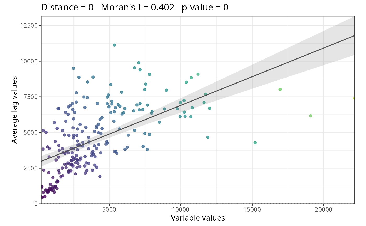
Moran's scatterplot:
The plot shows original values (x-axis) against spatially lagged values (y-axis). The slope of the fitted line approximates Moran's I. Points in quadrants I and III indicate positive spatial autocorrelation; points in quadrants II and IV indicate negative spatial autocorrelation.
This implementation is inspired by the Moran.I() function in the ape package.
See also
moran_multithreshold(), get_moran()
Other spatial_analysis:
filter_spatial_predictors(),
mem(),
mem_multithreshold(),
moran_multithreshold(),
pca(),
pca_multithreshold(),
rank_spatial_predictors(),
residuals_diagnostics(),
residuals_test(),
select_spatial_predictors_recursive(),
select_spatial_predictors_sequential()
Examples
data(plants_df, plants_distance, plants_response)

# Test for spatial autocorrelation in response variable
moran_test <- moran(
  x = plants_df[[plants_response]],
  distance.matrix = plants_distance,
  distance.threshold = 1000
)


# View test results
moran_test$test
#>   distance.threshold moran.i.null   moran.i p.value
#> 1               1000 -0.004424779 0.2588432       0
#>                 interpretation
#> 1 Positive spatial correlation

# Access components
moran_test$test$moran.i  # Observed Moran's I
#> [1] 0.2588432
moran_test$test$p.value  # P-value
#> [1] 0
moran_test$test$interpretation  # Text interpretation
#> [1] "Positive spatial correlation"
# View test results
moran_test$test
#> distance.threshold moran.i.null moran.i p.value
#> 1 1000 -0.004424779 0.2588432 0
#> interpretation
#> 1 Positive spatial correlation
# Access components
moran_test$test$moran.i # Observed Moran's I
#> [1] 0.2588432
moran_test$test$p.value # P-value
#> [1] 0
moran_test$test$interpretation # Text interpretation
#> [1] "Positive spatial correlation"