Plots the response surfaces of a random forest model

Plots response surfaces for any given pair of predictors in a rf(), rf_repeat(), or rf_spatial() model.

plot_response_surface(
  model = NULL,
  a = NULL,
  b = NULL,
  quantiles = 0.5,
  grid.resolution = 100,
  point.size.range = c(0.5, 2.5),
  point.alpha = 1,
  fill.color = viridis::viridis(100, option = "F", direction = -1, alpha = 0.9),
  point.color = "gray30",
  verbose = TRUE
)

Arguments

model

A model fitted with rf(), rf_repeat(), or rf_spatial(). Default NULL

a

Character string, name of a model predictor. If NULL, the most important variable in model is selected. Default: NULL

b

Character string, name of a model predictor. If NULL, the second most important variable in model is selected. Default: NULL

quantiles

Numeric vector between 0 and 1. Argument probs of the function quantile. Quantiles to set the other variables to. Default: 0.5

grid.resolution

Integer between 20 and 500. Resolution of the plotted surface Default: 100

point.size.range

Numeric vector of length 2 with the range of point sizes used by geom_point. Using c(-1, -1) removes the points. Default: c(0.5, 2.5)

point.alpha

Numeric between 0 and 1, transparency of the points. Setting it to 0 removes all points. Default: 1.

fill.color

Character vector with hexadecimal codes (e.g. "#440154FF" "#21908CFF" "#FDE725FF"), or function generating a palette (e.g. viridis::viridis(100)). Default: viridis::viridis(100, option = "F", direction = -1, alpha = 0.9)

point.color

Character vector with a color name (e.g. "red4"). Default: gray30

verbose

Logical, if TRUE the plot is printed. Default: TRUE

Value

A list with slots named after the selected quantiles, each one with a ggplot.

Details

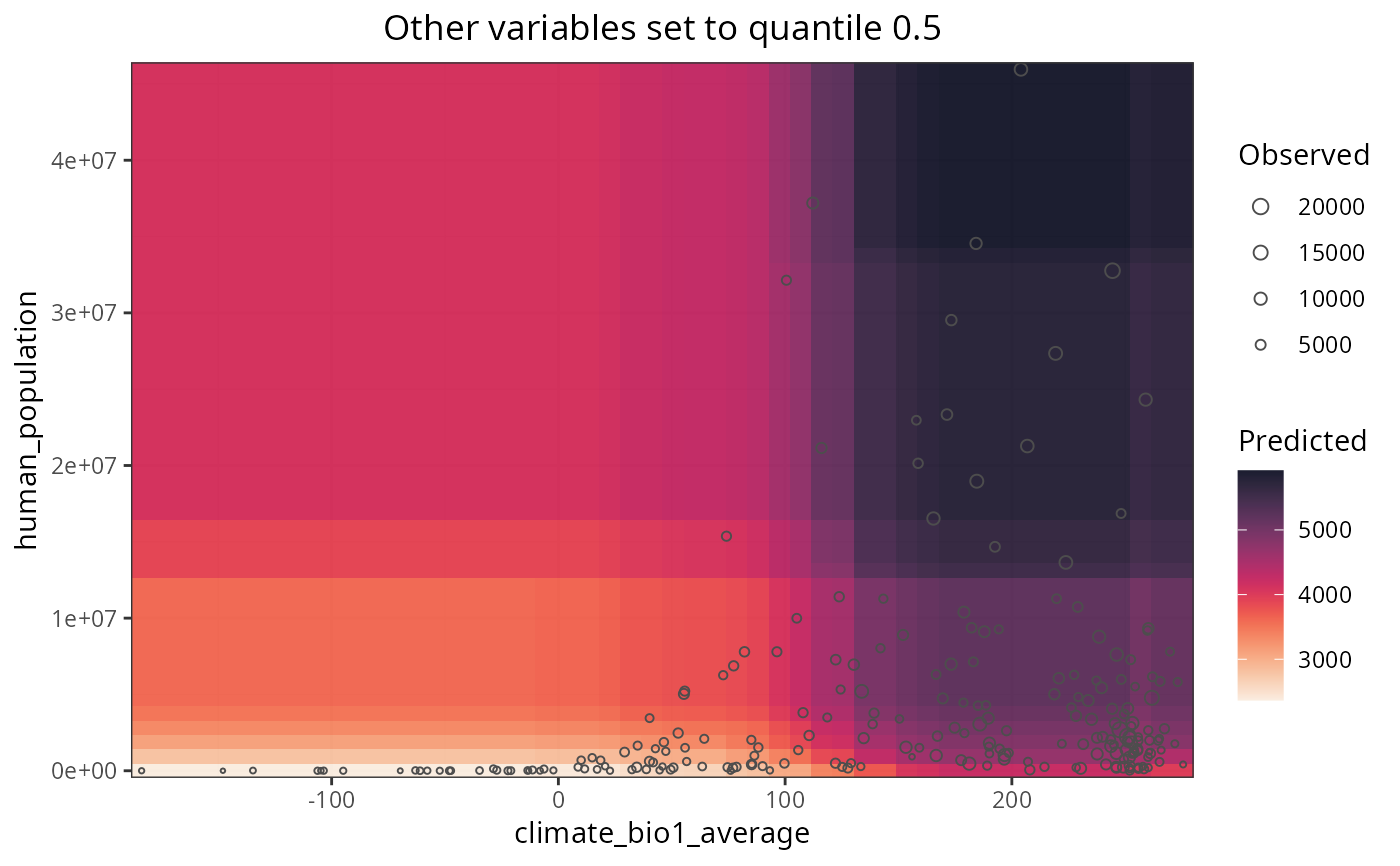
All variables that are not a or b in a response curve are set to the values of their respective quantiles to plot the response surfaces. The output list can be plotted all at once with patchwork::wrap_plots(p) or cowplot::plot_grid(plotlist = p), or one by one by extracting each plot from the list.

See also

plot_response_curves()

Examples

if(interactive()){

#load example data
data(plant_richness_df)

#fit random forest model
out <- rf(
 data = plant_richness_df,
 dependent.variable.name = "richness_species_vascular",
 predictor.variable.names = colnames(plant_richness_df)[5:21],
 n.cores = 1,
 verbose = FALSE
)

#plot interactions between most important predictors
plot_response_surfaces(x = out)


}