Random forest models with Moran's I test of the residuals

Fits a random forest model using ranger and extends it with spatial diagnostics: residual autocorrelation (Moran's I) at multiple distance thresholds, performance metrics (RMSE, NRMSE via root_mean_squared_error()), and variable importance scores computed on scaled data (via scale).

Usage

rf(
  data = NULL,
  dependent.variable.name = NULL,
  predictor.variable.names = NULL,
  distance.matrix = NULL,
  distance.thresholds = NULL,
  xy = NULL,
  ranger.arguments = NULL,
  scaled.importance = FALSE,
  seed = 1,
  verbose = TRUE,
  n.cores = parallel::detectCores() - 1,
  cluster = NULL
)

Arguments

data: Data frame with a response variable and a set of predictors. Default: NULL
dependent.variable.name: Character string with the name of the response variable. Must be a column name in data. For binary response variables (0/1), case weights are automatically computed using case_weights() to balance classes. Default: NULL
predictor.variable.names: Character vector with predictor variable names. All names must be columns in data. Alternatively, accepts the output of auto_cor() or auto_vif() for automated variable selection. Default: NULL
distance.matrix: Square matrix with pairwise distances between observations in data. Must have the same number of rows as data. If NULL, spatial autocorrelation of residuals is not computed. Default: NULL
distance.thresholds: Numeric vector of distance thresholds for spatial autocorrelation analysis. For each threshold, distances below that value are set to zero when computing Moran's I. If NULL, defaults to seq(0, max(distance.matrix), length.out = 4). Default: NULL
xy: Data frame or matrix with two columns containing coordinates, named "x" and "y". Not used by this function but stored in the model for use by rf_evaluate() and rf_tuning(). Default: NULL
ranger.arguments: Named list with ranger arguments. Arguments for this function can also be passed here. The default importance method is 'permutation' instead of ranger's default 'none'. The x, y, and formula arguments are not supported. See ranger help for available arguments. Default: NULL
scaled.importance: If TRUE, variable importance is computed on scaled data using scale, making importance scores comparable across models with different predictor units. Default: FALSE
seed: Random seed for reproducibility. Default: 1
verbose: If TRUE, display messages and plots during execution. Default: TRUE
n.cores: Number of cores for parallel execution. Default: parallel::detectCores() - 1
cluster: Cluster object from parallel::makeCluster(). Not used by this function but stored in the model for use in downstream functions. Default: NULL

Value

A ranger model object with additional slots:

ranger.arguments: Arguments used to fit the model.
importance: List with global importance data frame (predictors ranked by importance), importance plot, and local importance scores (per-observation difference in accuracy between permuted and non-permuted predictors, based on out-of-bag data).
performance: Model performance metrics including R-squared (out-of-bag and standard), pseudo R-squared, RMSE, and NRMSE.
residuals: Model residuals with normality diagnostics (residuals_diagnostics()) and spatial autocorrelation (moran_multithreshold()).

Details

See ranger documentation for additional details. The formula interface is supported via ranger.arguments, but variable interactions are not permitted. For feature engineering including interactions, see the_feature_engineer().

Examples


data(
  plants_df,
  plants_response,
  plants_predictors,
  plants_distance
)

m <- rf(
  data = plants_df,
  dependent.variable.name = plants_response,
  predictor.variable.names = plants_predictors,
  distance.matrix = plants_distance,
  distance.thresholds = c(100, 1000, 2000),
  ranger.arguments = list(
    num.trees = 50,
    min.node.size = 20
  ),
  verbose = FALSE,
  n.cores = 1
)

class(m)
#> [1] "rf"     "ranger"
#variable importance
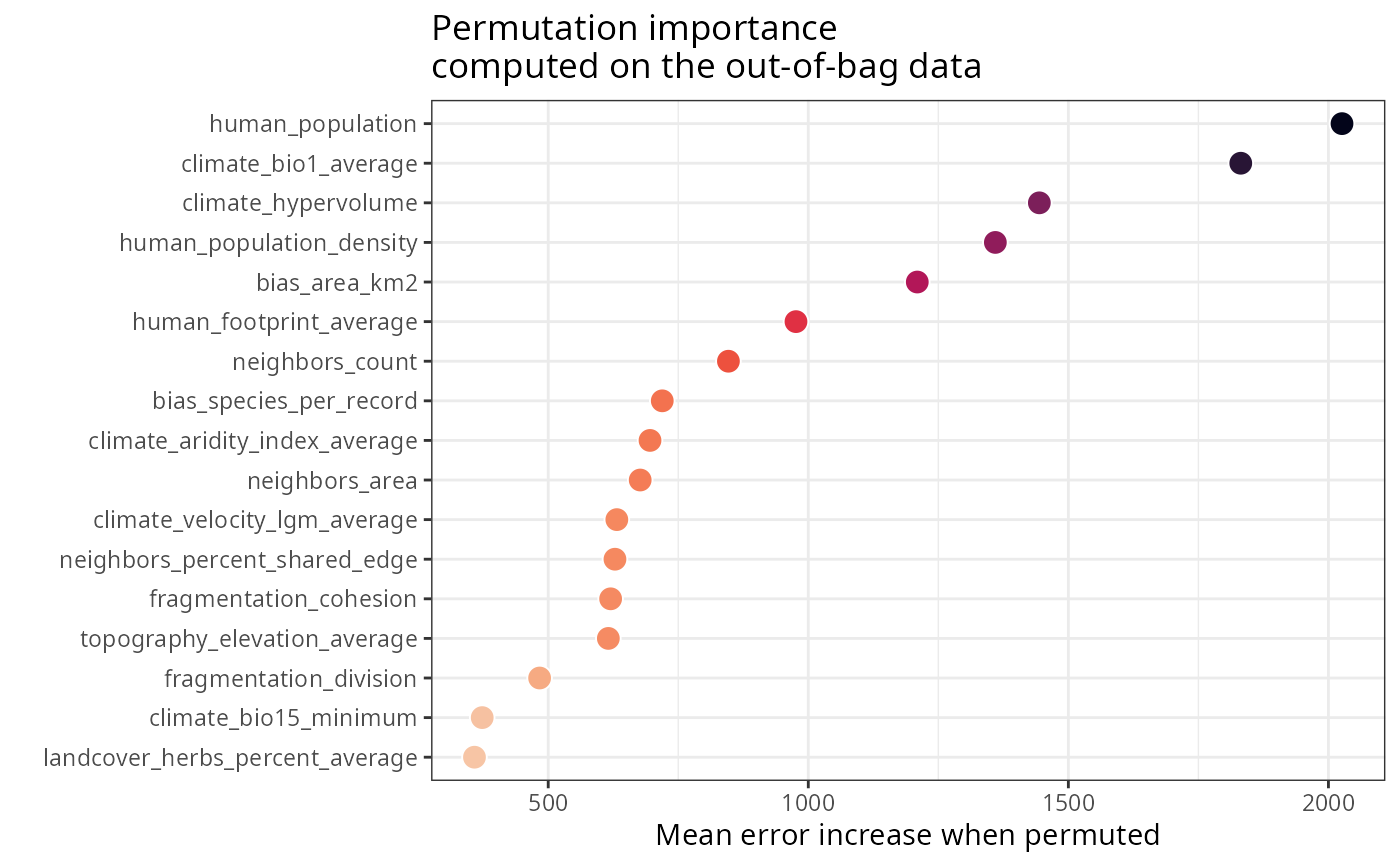
m$importance$per.variable
#>                           variable importance
#> 1             climate_bio1_average   1862.351
#> 2                 human_population   1602.213
#> 3          human_footprint_average   1348.596
#> 4              climate_hypervolume   1340.019
#> 5                    bias_area_km2   1165.371
#> 6         human_population_density   1040.106
#> 7                  neighbors_count    826.140
#> 8          bias_species_per_record    824.618
#> 9                   neighbors_area    694.325
#> 10   climate_aridity_index_average    673.057
#> 11    topography_elevation_average    650.577
#> 12          fragmentation_cohesion    507.302
#> 13    climate_velocity_lgm_average    459.043
#> 14   neighbors_percent_shared_edge    289.154
#> 15 landcover_herbs_percent_average    277.146
#> 16          fragmentation_division    216.471
#> 17           climate_bio15_minimum     83.932
m$importance$per.variable.plot


#model performance
m$performance
#> $r.squared.oob
#> [1] 0.5317319
#> 
#> $r.squared
#> [1] 0.8737717
#> 
#> $pseudo.r.squared
#> [1] 0.9347576
#> 
#> $rmse.oob
#> [1] 2306.124
#> 
#> $rmse
#> [1] 1431.987
#> 
#> $nrmse
#> [1] 0.4133911
#> 
#> $auc
#> [1] NA
#> 

#autocorrelation of residuals
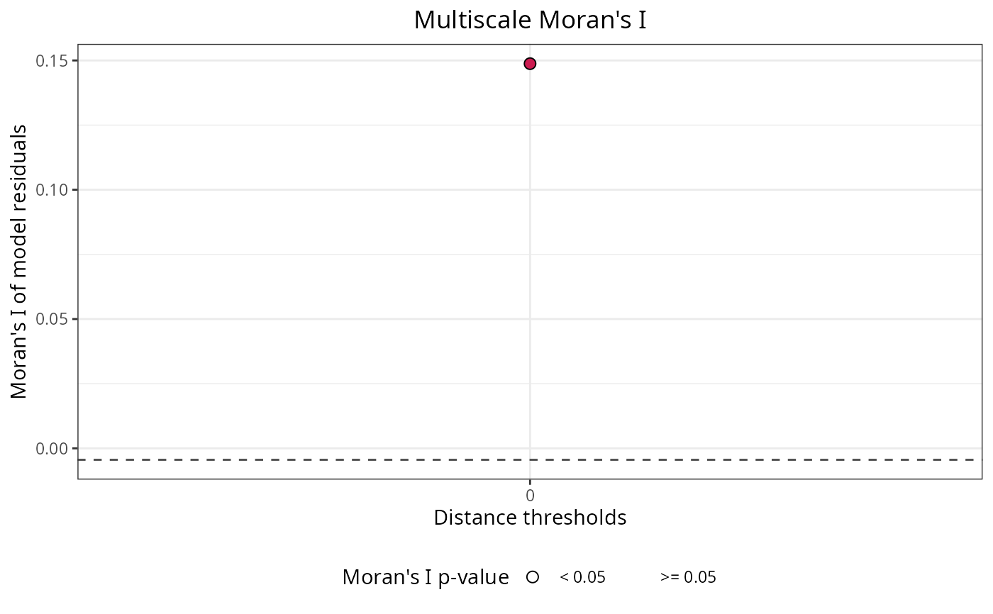
m$residuals$autocorrelation$per.distance
#>   distance.threshold    moran.i moran.i.null      p.value
#> 1                100 0.13056941 -0.004424779 1.348179e-05
#> 2               1000 0.06011484 -0.004424779 2.425928e-05
#> 3               2000 0.01931070 -0.004424779 1.781684e-02
#>                 interpretation
#> 1 Positive spatial correlation
#> 2 Positive spatial correlation
#> 3 Positive spatial correlation
m$residuals$autocorrelation$plot


#model predictions
m$predictions$values
#>   [1]  5291.4899  5578.2987  1589.6221  7102.8035 10067.5064  3055.0196
#>   [7]  4954.8124  5759.2277  2948.4820  4335.4926  3102.5294  2873.0971
#>  [13]   802.9309  5814.4622  7004.7033  6894.4869  3719.2509  4470.5535
#>  [19]  6649.0718  3324.5036  5768.4359  5656.5501 10388.7945  2748.6759
#>  [25]   682.9654  6353.5133  2717.0396  2356.0581  1417.0340  1602.4763
#>  [31]  3935.2395  6611.4979  4166.2661  2917.4196  8102.2748  7190.4895
#>  [37]  2721.3488  2831.5914   884.4582  1228.9204  3061.8315  3246.7019
#>  [43]  3066.1162  4477.7483  3839.9562  4033.3966  2497.9233  1837.6491
#>  [49]  1983.3319  3717.5131  5813.2443  3141.5729  1419.2481  3085.4385
#>  [55]   776.2131  9853.9472  4719.6057  3017.3389  2208.1689   975.1962
#>  [61]  2713.6945  2841.2230  9292.8148  5349.9251  3004.0502  3597.7268
#>  [67]  9496.7950  4233.8299  1469.4442  3787.3333  4192.5505  1146.0211
#>  [73]  7692.6330  5274.9740  6076.2094  1468.0671  2362.9449  1788.2738
#>  [79]  2044.7630  3817.0928  2140.2234  1369.7570  3360.5352  3584.7737
#>  [85]  3759.0037   870.7700  2877.5964  2794.6387  2908.1380  2389.2811
#>  [91]  5849.2702  1532.3995  1952.5626  8642.1687  4077.2436  4276.5161
#>  [97]  7539.0082  6939.6704  9257.4595  3132.0103  2698.9396  5404.9854
#> [103]  1721.5442  2742.1876  3236.3743  2903.9876  6739.2454  5173.7660
#> [109]  6587.8270  1558.1043  2445.5070  3438.7889  3195.8107  3218.5243
#> [115]  6712.7303  1053.8067  2439.9376  2227.9587  3656.7509   926.8010
#> [121]  2927.1745  9464.9285  1179.5736  3423.5251  3999.9025  5645.2067
#> [127]  3915.2952  4057.6235  2689.2356  3785.8296  4984.9734  2784.1061
#> [133]  1043.4002  5023.7544  6176.3488  7278.0910  1052.5757  2577.6017
#> [139]  3403.8022  1282.3107  6526.7393  3005.8826  1206.0567  6148.5235
#> [145]  4843.7370  2113.5744  3573.0392  5528.7805  1521.9094   957.6785
#> [151]  3205.5720  2486.5204  6020.9469  2415.1661  6540.9665  6351.5947
#> [157]  7411.1992  3438.1847  3487.1045  7703.7450  3910.5639  2336.9264
#> [163]  4853.1863  7826.6064 12477.2066  2677.8060  5003.5714  2184.9405
#> [169]  2162.6979  2455.8144  6643.7121  1011.8905  1677.4915  4935.4205
#> [175]  3339.3278  3808.0361  3122.7009 12272.9463  2791.2426   954.0983
#> [181]  5271.1207  6339.4611   695.3549  3921.9516  6532.4750  3177.0817
#> [187]  5130.8285  8334.9741  4767.9979  4567.5731  4603.0198  8692.9414
#> [193]  5332.1238  6047.4604  9424.3609   833.4410   796.6555 10944.7190
#> [199]  2488.9519  1804.4019  3270.6800  3642.4388  6057.9466  7303.2465
#> [205]  4181.6663  4271.4106  6505.1590  2853.0312  2649.4218  1759.4082
#> [211]  2922.7903  2891.5668  5442.8218  7670.3069  5776.2621  7013.3065
#> [217]  1767.0014  5127.4461  2833.0677  3159.8775  3361.5099  3585.5471
#> [223]  6777.3612  4934.7655  3729.7678  4813.3794  2553.2253

#predictions for new data (using stats::predict)
y <- stats::predict(
  object = m,
  data = plants_df[1:5, ],
  type = "response"
)$predictions

#alternative: pass arguments via ranger.arguments list
args <- list(
  data = plants_df,
  dependent.variable.name = plants_response,
  predictor.variable.names = plants_predictors,
  distance.matrix = plants_distance,
  distance.thresholds = c(100, 1000, 2000),
  num.trees = 50,
  min.node.size = 20,
  num.threads = 1
)

m <- rf(
  ranger.arguments = args,
  verbose = FALSE
)