Dynamic Time Warping vs Lock-Step • distantia

Summary

The R package distantia provides tools for comparing time series through two distinct methods: dynamic time warping (DTW) and lock-step (LS). These approaches cater to different analysis needs: DTW for handling temporal shifts and LS for preserving temporal alignment. This article explores the conceptual foundations of both methods, their implementation in distantia, and showcases their practical use with code examples.

Setup

The packages required to run the code in this article are distantia and dtw. The latter is not a dependency of distantia, but will help put into context key details of how DTW works.

Example data

The cities_temperature dataset contains monthly temperature records for 20 cities. The code below transforms it into a Time Series List (TSL) and selects a subset of three cities with temperature time series from 2000 to 2005.

tsl_raw <- tsl_initialize(
  x = cities_temperature,
  name_column = "name",
  time_column = "time"
) |> 
  tsl_subset(
    names = c(
      "London", 
      "Paris", 
      "Kinshasa"
    ),
    time = c(
      "2000-01-01", 
      "2005-01-01"
    )
  )

tsl_plot(
  tsl = tsl_raw,
  ylim = "relative"
)

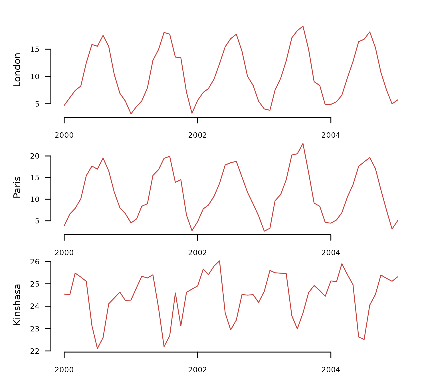
The transformed TSL contains two synchronous time series in the Northern Hemisphere with similar temperature ranges (London and Paris) and one in the Southern Hemisphere (Kinshasa) with a higher average and a shifted temporal pattern.

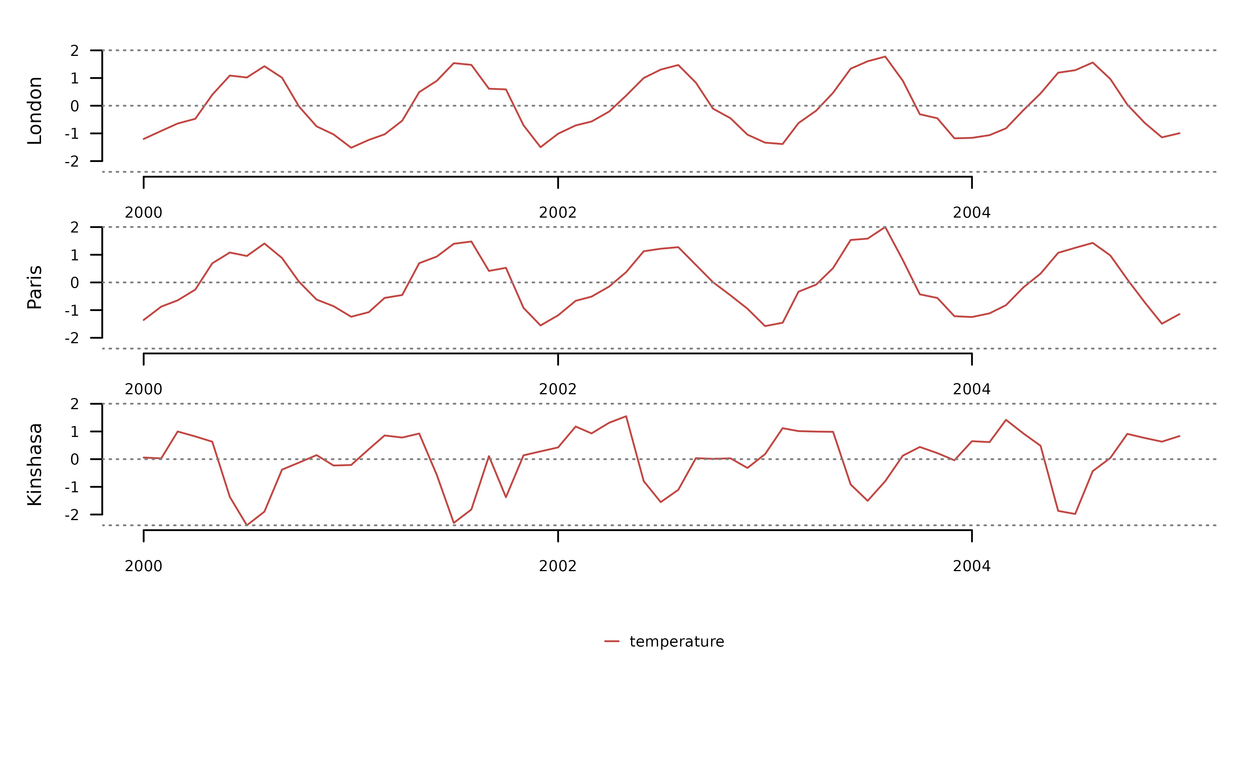
To facilitate the comparison of DTW and LS, the code below applies the functions tsl_transform() and f_scale apply local (each time series is scaled separately) centering and scaling to the data.

tsl_scaled <- tsl_transform(
  tsl = tsl_raw,
  f = f_scale_local,
  center = TRUE,
  scale = TRUE
)

tsl_plot(
  tsl = tsl_scaled
)

Lock-Step (LS)

Lock-step methods compare values at corresponding time points, requiring time series of the same length sampled at identical times. This approach is well-suited for cases where maintaining the temporal alignment of the compared time series is crucial. The method is straightforward and computationally efficient.

In distantia, lock-step comparisons are carried out in three steps:

1.- Sum the distances between pairs of samples observed at the same times.

2.- Sum the distances between consecutive samples within each time series.

3.- Compute the normalized dissimilarity score psi.

Let’s look first at a native R implementation of this idea using euclidean distances to keep it simple.

#extracting the data to shorten variable names
x <- tsl_scaled$London
y <- tsl_scaled$Kinshasa

#1.- sum of distances between pairs of samples
step_1 <- sum(sqrt((x - y)^2))

#2.- sum of distances between consecutive samples
step_2 <- sum(
  sqrt(diff(x)^2) + sqrt(diff(y)^2)
  )

#3.- compute normalized dissimilarity score
((2 * step_1) / step_2)
#> [1] 2.792455

The function distantia() performs the same task when lock_step = TRUE (default is FALSE).

df <- distantia(
  tsl = tsl_scaled[c("London", "Kinshasa")],
  lock_step = TRUE,
  distance = "euclidean"
)

df$psi
#> [1] 2.792455

The function distantia() can compute lock-step dissimilarity scores for time series in tsl at once.

df_LS <- distantia(
  tsl = tsl_scaled,
  lock_step = TRUE
)
df_LS[, c("x", "y", "psi")]
#>        x        y       psi
#> 1 London    Paris 0.2427342
#> 3  Paris Kinshasa 2.7153379
#> 2 London Kinshasa 2.7924554

As expected, London and Paris show the most similar temperature time series, while London and Kinshasa are the most different ones.

Dynamic Time Warping

Dynamic Time Warping (DTW) aligns the time axes of two time series to maximize pattern similarity, even when temporal shifts are present. This makes DTW ideal for comparing time series with similar shapes but misaligned time points. However, it is computationally more intensive and less efficient than the lock-step method, particularly for large datasets.

DTW involves three conceptual steps, similar to the lock-step method, but with additional complexity in the first step:

1.- Sum the distances between pairs of samples.

1a Compute a distance matrix between all pairs of samples.
1b Build the least-cost matrix.
1c Find the least-cost path.
1d Sum distances along the least-cost path.

2.- Sum distances between consecutive samples within each time series.

3.- Calculate the normalized dissimilarity score psi (with a slightly different formula!).

Now, let’s dive into the code.

The objective of the step 1 is computing the sum of distances between pairs of samples matched together by the time warping algorithm.

Step 1a computes the distance matrix between all pairs of samples in both timme series. Notice that all functions to demonstrate the computation of the normalized dissimilarity score psi follow the naming convention psi...().

m.dist <- psi_distance_matrix(
  x = x,
  y = y,
  distance = "euclidean"
)

utils_matrix_plot(
  m = m.dist,
  diagonal_width = 0
  )

Step 1b involves transforming the distance matrix into a cost matrix. This transformation requires a dynamic algorithm in which each new cell adds its own distance to the distance accumulated by its preceding neighbor. There are two implementations of this method in distantia:

orthogonal only: distance cost is only computed on the x and y axis, ignoring diagonals.
orthogonal and diagonal: distance cost is also computed in diagonals, which are weighted by a factor of 1.414214.

These options are wrapped in the function psi_cost_matrix(), which by default, like distantia() uses weighted diagonals.

m.cost <- psi_cost_matrix(
  dist_matrix = m.dist,
  diagonal = TRUE #default
)

utils_matrix_plot(
  m = m.cost,
  diagonal_width = 0
  )

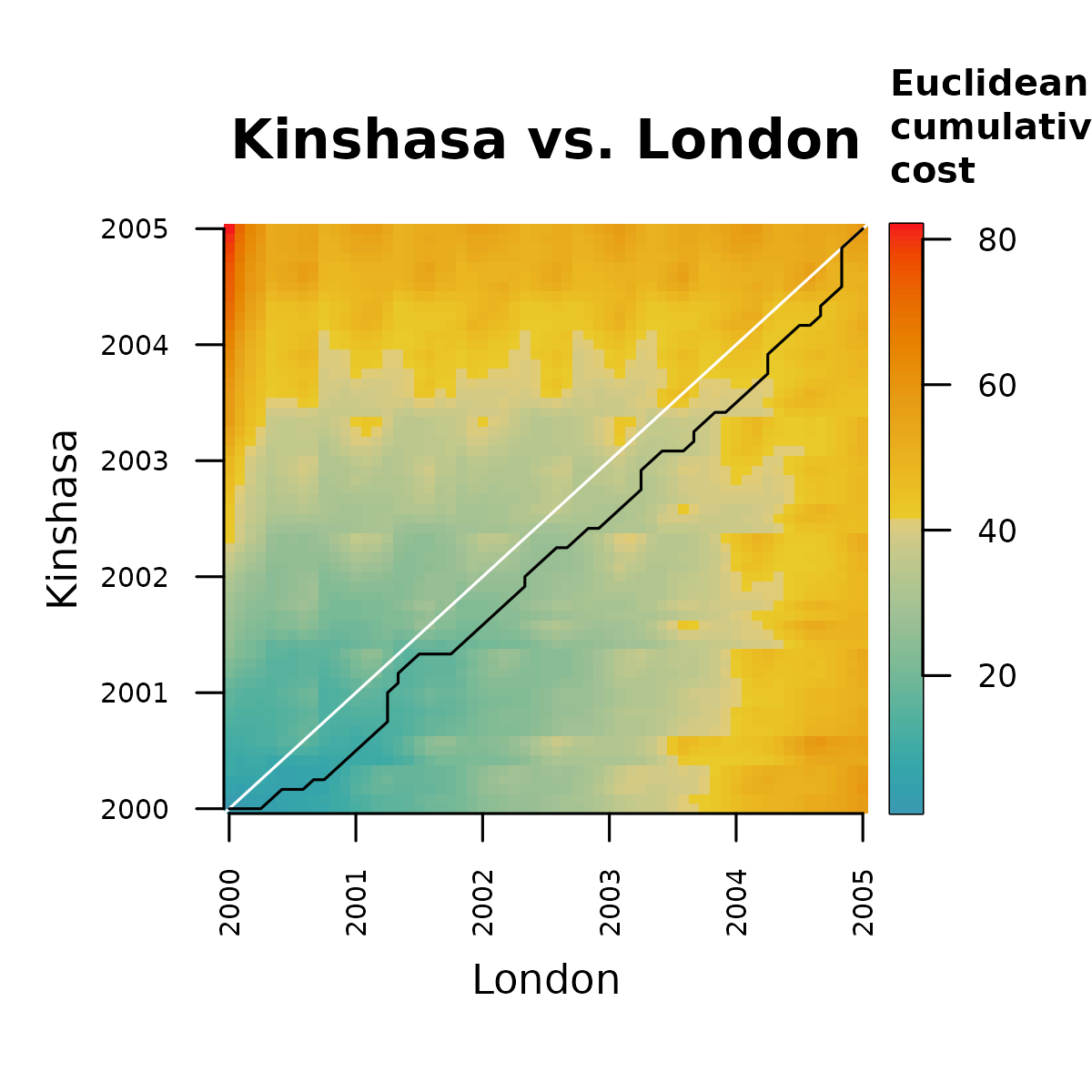
In step 1c, the distance and cost matrices are used to find the least-cost path.

m.cost.path <- psi_cost_path(
  dist_matrix = m.dist,
  cost_matrix = m.cost,
  diagonal = TRUE #default
)

tail(m.cost.path)
#>    x y       dist     cost
#> 73 6 3 0.09001854 4.820301
#> 74 5 2 0.36818140 4.126921
#> 75 4 1 0.53175876 3.460522
#> 76 3 1 0.70059611 2.928764
#> 77 2 1 0.96840001 2.228167
#> 78 1 1 1.25976738 1.259767

Notice that the cost path data frame is ordered from bottom to top. The columns “x” and “y” represent sample indices of the time series London and Kinshasa. The figure below shows the least cost path on top of the cost matrix.

utils_matrix_plot(
  m = m.cost,
  path = m.cost.path
)

The step 1d finalizes the DTW logic by adding the distances between pair of samples connected by the least-cost path. This step is just sum(m.cost.path$dist), but it is implemented in psi_cost_path_sum(), which also checks that the least cost data frame is correct.

step_1 <- psi_cost_path_sum(
  path = m.cost.path
)

step_1
#> [1] 39.44194

Step 2 returns the distances between consecutive samples within each time series, as computed by psi_auto_sum().

step_2 <- psi_auto_sum(
  x = x,
  y = y,
  distance = "euclidean"
)

step_2

Finally, the step 3 computes the normalized dissimilarity score.

psi_equation(
  a = step_1,
  b = step_2,
  diagonal = TRUE
)

All these individual steps can be performed at once with the function distantia() by setting the argument lock_step to FALSE.

df <- distantia(
  tsl = tsl_scaled[c("London", "Kinshasa")],
  lock_step = FALSE,
  distance = "euclidean"
)

df[, c("x", "y", "psi")]
#>        x        y      psi
#> 1 London Kinshasa 1.153969

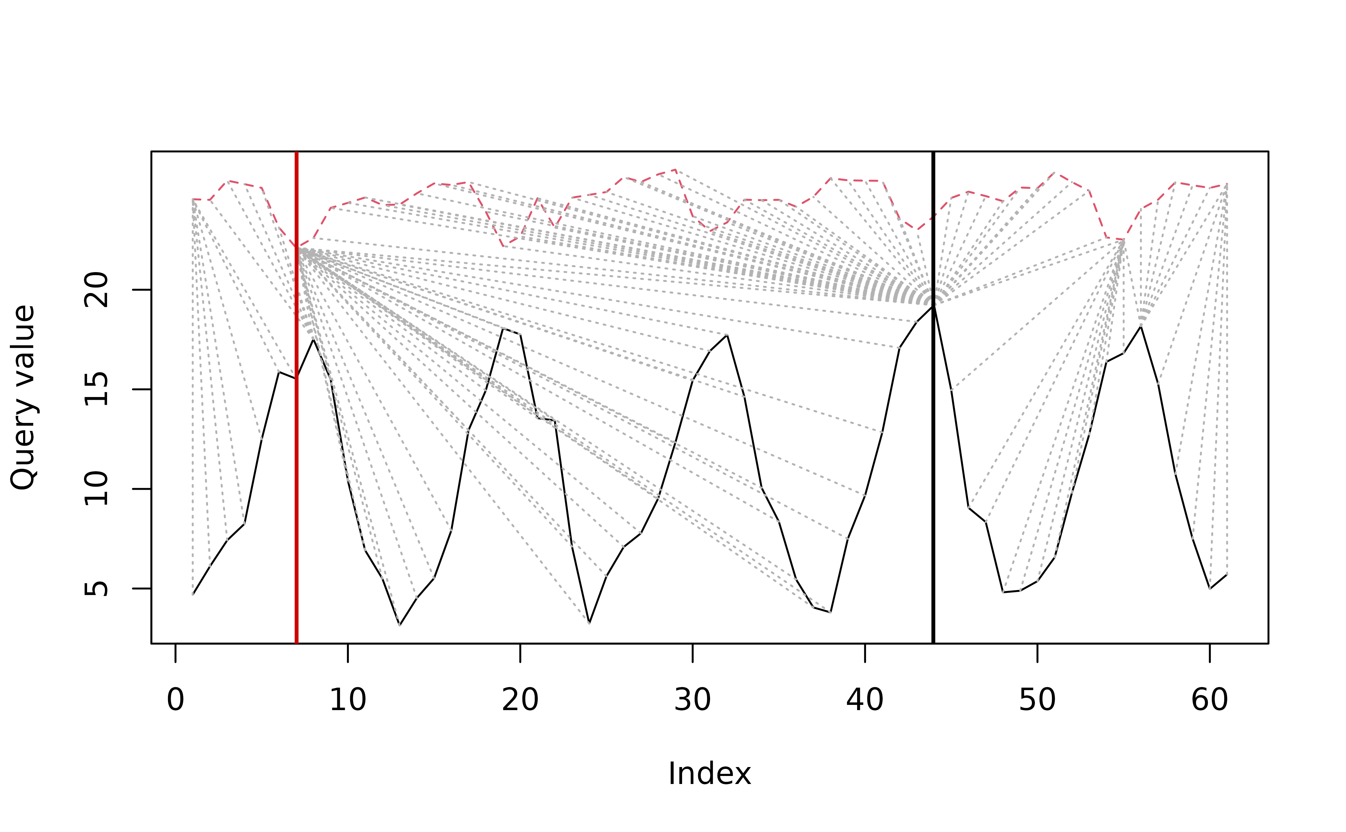
The function distantia_plot() offers a good graphical representation of the warping result and decomposes the computation of the psi dissimilarity score.

distantia_plot(
  tsl = tsl_scaled[c("London", "Kinshasa")]
)

Pitfalls

DTW is an ideal method to compare time series with temporal shifts, and is applicable to regular and irregular time series with the same or different numbers of samples.

However, DTW is highly sensitive to differences in data magnitudes. As result, data that is not properly scaled may distort the warping, leading to .

The plot below represents the DTW alignment of London and Kinshasa on the raw temperature data. It shows how DTW gets stuck in two local optima, one in the y axis (long horizontal line) at the minimum temperature in Kinshasa (winter of 2001), and another in the x axis (long vertical line) at the maximum temperature in London (summer of 2003). It also shows a distinctively large dissimilarity score.

distantia_plot(
  tsl = tsl_raw[c("London", "Kinshasa")]
)

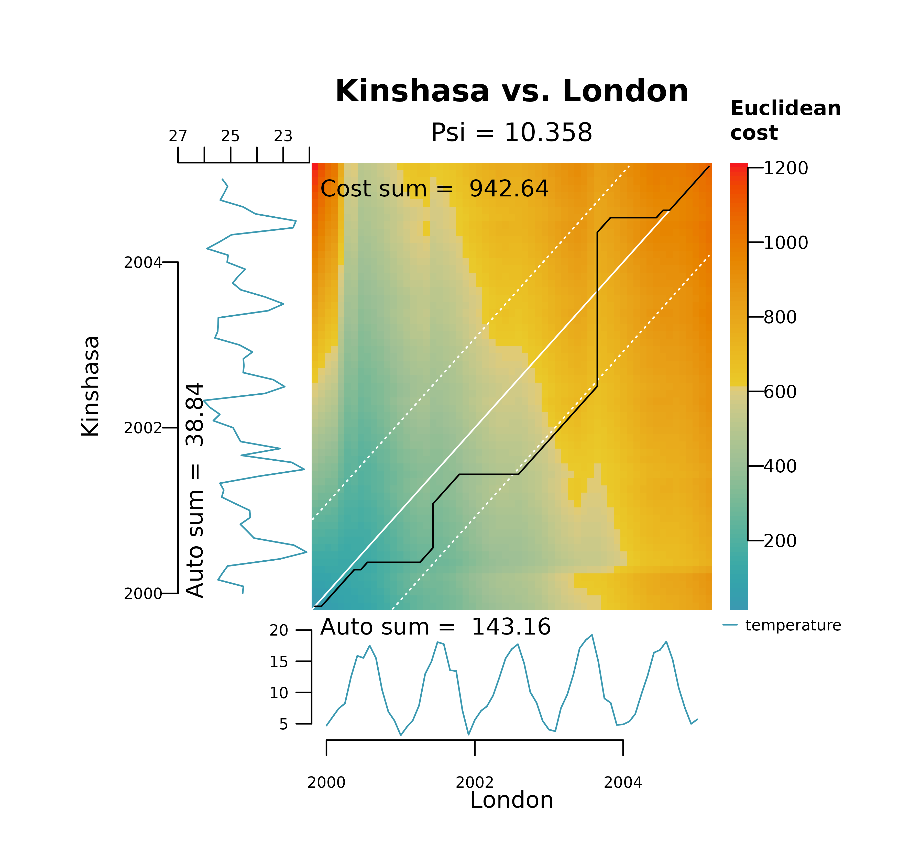
These long horizontal and vertical lines shown above provide an immediate diagnostic of the issue.

This is not a particular issue of the DTW algorithm implemented in distantia, but a general behavior of time warping methods. The code below shows a similar analysis performed with the R package dtw. The default implementation ignores diagonals when building the cost matrix.

xy_dtw <- dtw::dtw(
  x = tsl_raw$London$temperature,
  y = tsl_raw$Kinshasa$temperature,
  keep = TRUE
  )

plot(xy_dtw, type = "threeway")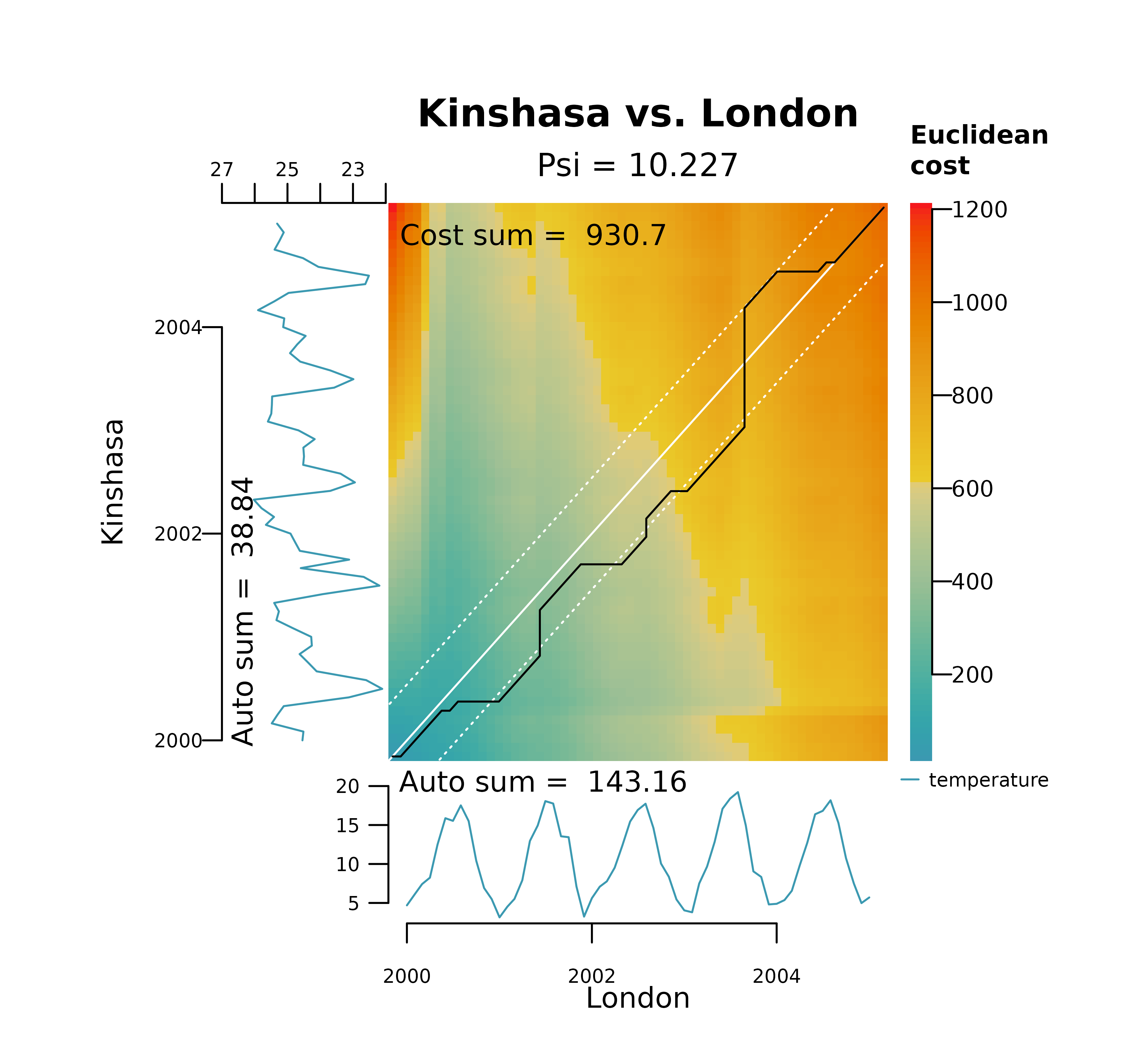

The “twoway” plot provided by dtw shows the alingment as a line bar, with the sample matches represented as dotted lines, and two vertical lines highlighting the local optima

plot(xy_dtw, type = "twoway")
abline(v=0.13, col="red3", lwd = 2)
abline(v=0.70, col="black", lwd = 2)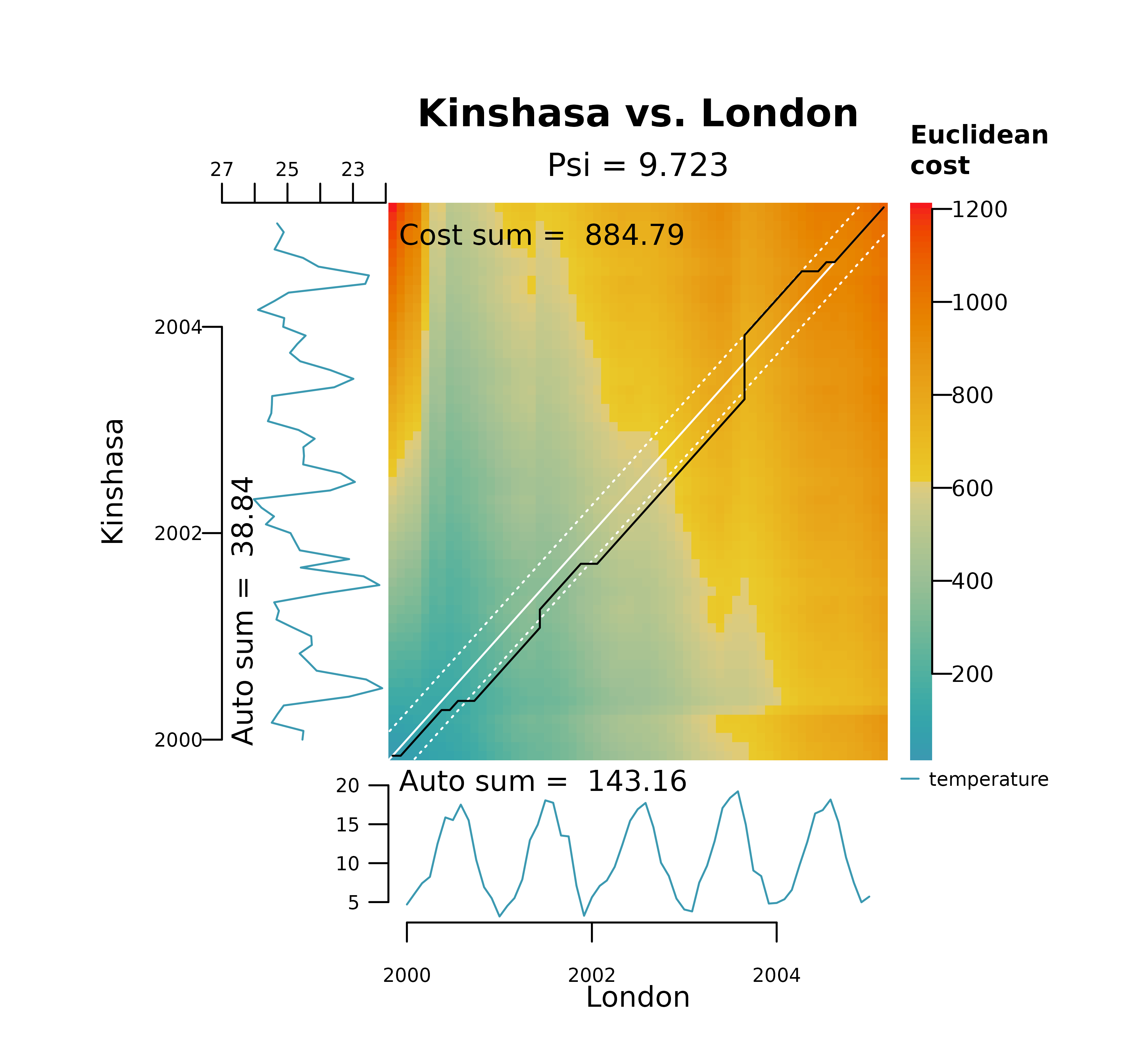

There are two strategies that can be combined to control this issue: data scaling, and constrained DTW.

Constrained DTW

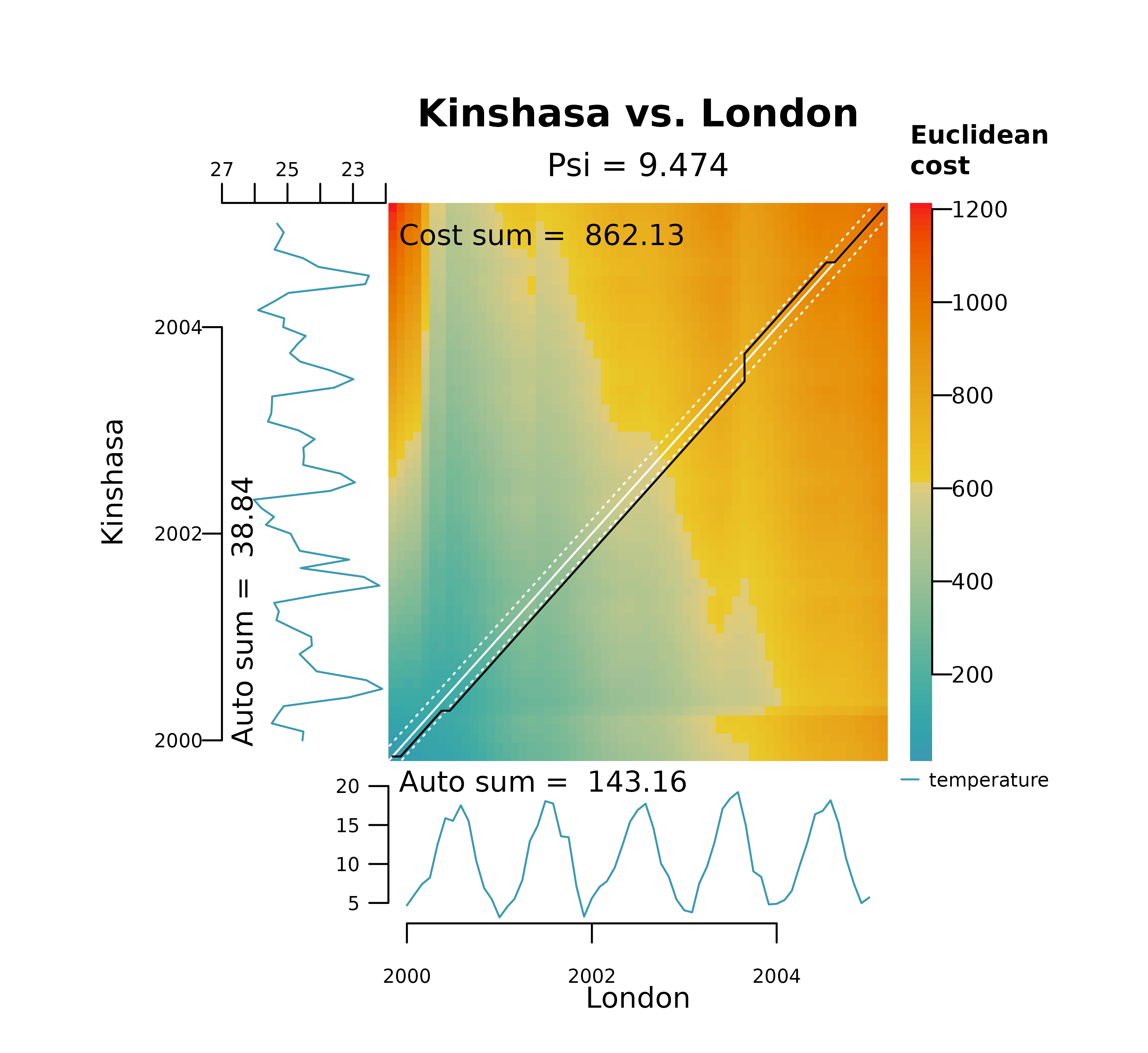
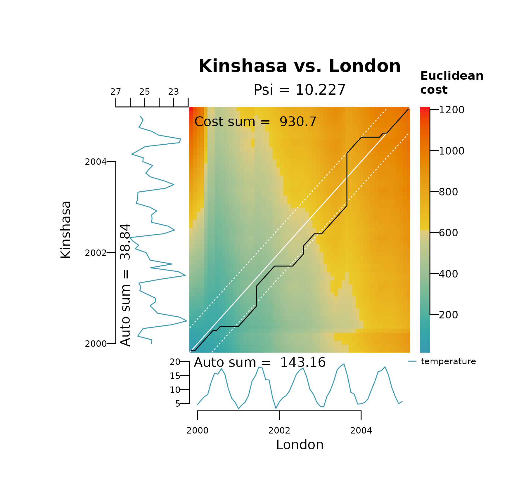
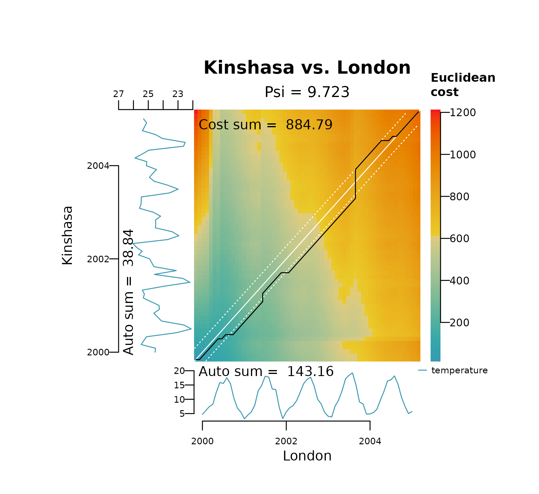
The function distantia() implements Itakura parallelograms to restrict the flexibility of the warping path via the bandwidth argument. This argument represents the fraction of space at both sides of the least cost matrix diagonal allowed for warping. The plots below show the effect of decreasing bandwidth on the area covered by the Itakura parallelograms (shown as white dashed lines) and how it restricts spread of the alignment between London and Kinshasa on their raw temperature values.

distantia_plot(
  tsl = tsl_raw[c("London", "Kinshasa")],
  bandwidth = 0.2
)

distantia_plot(
  tsl = tsl_raw[c("London", "Kinshasa")],
  bandwidth = 0.1
)

distantia_plot(
  tsl = tsl_raw[c("London", "Kinshasa")],
  bandwidth = 0.05
)

distantia_plot(
  tsl = tsl_raw[c("London", "Kinshasa")],
  bandwidth = 0.025
)

Itakura parallelograms cannot fix bad alignments (that’s what data scaling is for), but can help diagnose them, given a tolerance level.

The code below runs distantia() for the raw temperature data with two bandwidths: 1 for unrestricted dynamic time warping, and 0.25 as reference level.

df <- distantia(
  tsl = tsl_raw,
  bandwidth = c(1, 0.25)
)

df[, c("x", "y", "psi", "bandwidth")]
#>        x        y        psi bandwidth
#> 1 London    Paris  0.4422241      1.00
#> 4 London    Paris  0.4422241      0.25
#> 3  Paris Kinshasa  7.2974857      1.00
#> 6  Paris Kinshasa  7.6164475      0.25
#> 5 London Kinshasa 10.2968144      0.25
#> 2 London Kinshasa 10.7168885      1.00

Now, we can compute the psi differences across bandwidths for each pair of time series

df |> 
  dplyr::group_by(
    x, y
  ) |> 
  dplyr::summarise(
    psi_diff = diff(psi)
  )
#> `summarise()` has grouped output by 'x'. You can override using the `.groups`
#> argument.
#> # A tibble: 3 × 3
#> # Groups:   x [2]
#>   x      y        psi_diff
#>   <chr>  <chr>       <dbl>
#> 1 London Kinshasa    0.420
#> 2 London Paris       0    
#> 3 Paris  Kinshasa    0.319

All pairs of time series with a psi_diff higher than zero show warping paths that go beyond the 0.25 bandwidth.

Comparing DTW and LS

Dynamic Time Warping (DTW) and Lock-Step (LS) methods differ in scope and application.

DTW is ideal for comparing data that may be shifted in time due to positional differences, such as phenological time series observed across different hemispheres or elevations. It also facilitates the comparison of time series with varying lengths, observation periods, or sampling resolutions. This versatility makes DTW a general-purpose tool for time series analysis.

In contrast, LS is designed for synchronized time series that, at a minimum, must have the same length. While its scope is narrower, LS is more intuitive and accurate than DTW for comparing time series without time shifts, as it measures raw differences directly.

In essence, DTW, with its ability to adjust the time axis, answers the question, How similar can these two time series be?, while LS addresses the question, “How different are these two time series?”

The code below computes the dissimilarity score of the temperatures in Paris, London, and Kinshasa using DTW and LS and compares them in a data frame.

df_dtw <- distantia(
  tsl = tsl_scaled
)

df_ls <- distantia(
  tsl = tsl_scaled,
  lock_step = TRUE
)

data.frame(
  x = df_dtw$x,
  y = df_dtw$y,
  psi_dtw = round(df_dtw$psi, 3),
  psi_ls = round(df_ls$psi, 3)
)
#>        x        y psi_dtw psi_ls
#> 1 London    Paris   0.223  0.243
#> 2 London Kinshasa   1.154  2.715
#> 3  Paris Kinshasa   1.178  2.792

For London and Paris, both DTW and LS show very similar values, because the time series are very similar and DTW cannot do much else to adjust them even more. On the other hand, DTW shows much lower values than LS when Kinshasa comes into play, as it compensates the seasonal shifts in these time series. In that sense, LS provides a more accurate image of the raw differences between these time series.

As a clear advantage, LS does not require data normalization for univariate time series, and therefore can provide a dissimilarity score in the same units of the variable at hand.

df_ls <- distantia(
  tsl = tsl_raw,
  lock_step = TRUE
)

df_ls[, c("x", "y", "psi")]
#>        x        y       psi
#> 1 London    Paris 0.4879081
#> 3  Paris Kinshasa 7.5416106
#> 2 London Kinshasa 9.3361647

Comparing the dissimilarity scores above with the mean temperatures of the three cities below can give a sense of how approximate LS scores are to what we could expect.

df_stats <- tsl_stats(
  tsl = tsl_raw,
  lags = 0
)

df_stats[, c("name", "mean")]
#>       name     mean
#> 1   London 10.55682
#> 2    Paris 11.53803
#> 3 Kinshasa 24.48500

Closing Thoughts

The distantia package strikes a balance between flexibility and simplicity, enabling a more nuanced exploration of time series data. With support for both dynamic time warping and lock-step methods, it provides users with the tools needed to uncover insights while respecting the unique constraints of their data. Whether you’re working on sequence alignment or strict temporal comparisons, distantia is designed to adapt to your analytical needs.

I encourage you to give it a try and see how it fits into your workflows.