Getting Started
getting_started.RmdThis article walks through the complete memoria workflow
for quantifying ecological memory in time series data consisting of at
least one response and one predictor.
Ecological Memory
The package memoria helps quantify how past and
concurrent events shape the state of a system. This concept is
summarized in the figure below:
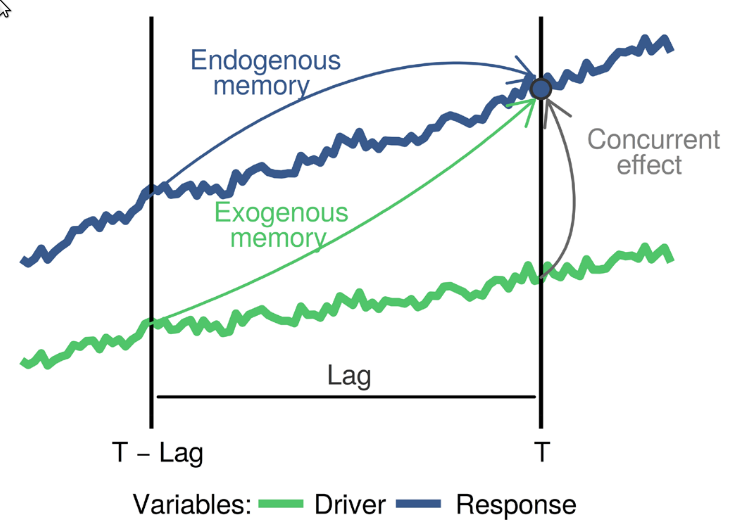 The blue
and green curves represent the values of a biotic response
The blue
and green curves represent the values of a biotic response
y and a driver x over time. The vertical line
T represents the current time, while
T - lag represents a previous time. The arrows represent
influence, as follows:
-
Endogenous memory: is the effect of past
yon presenty. -
Exogenous memory: is the effect of past
xon presenty. -
Concurrent effect: is the effect of present
xon presenty.
To assess these effects, memoria generates the lagged
data and trains the model
Where:
- and are the response and the driver.
- is the “current” time, and to , are the time lags.
- represents the endogenous memory across lags.
- represents the exogenous memory across lags.
- represents the concurrent effect.
- is a random term used to assess statistical significance.
The ecological memory pattern is quantified using permutation importance from Random Forest models. For each predictor, the algorithm shuffles its values and measures the decrease in predictive accuracy. Larger decreases indicate stronger influence on the response.
To visualize ecological memory, the package memoria
plots permutation importance scores across time lags.
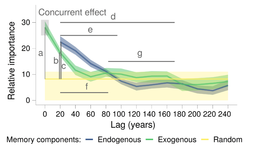
Where:
-
a: strength of the concurrent effect (highlighted by a grey box). -
bandc: strength of the exogenous and endogenous memory. -
dande: length of the exogenous and endogenous memory. -
fandg: dominance across lags of the endogenous and exogenous memory.
The following sections demonstrate how to implement this workflow in
R using the memoria package.
Workflow
The typical workflow involves time series with one response variable and one or several drivers.
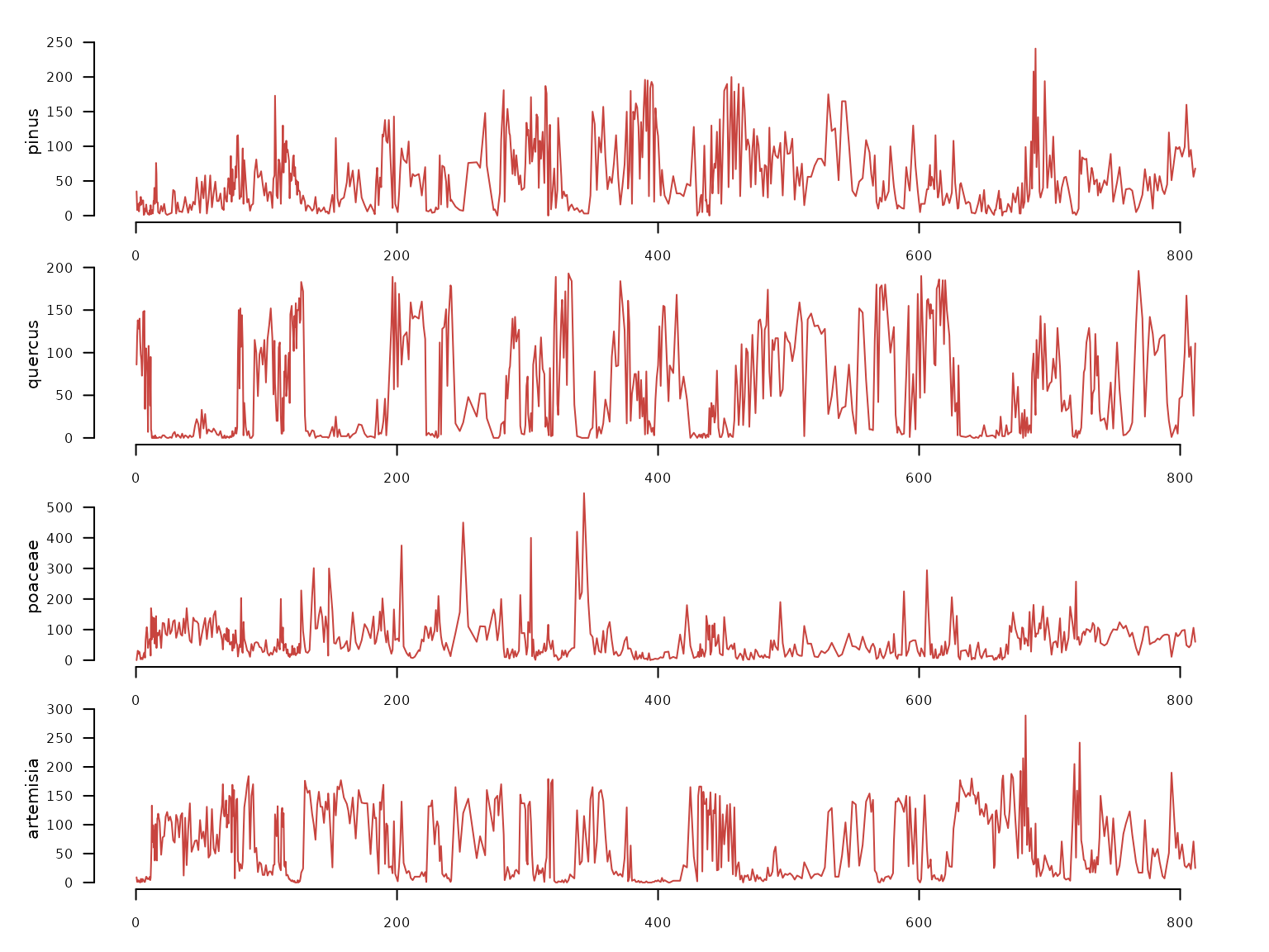
The package memoria has two example datasets, one with
responses and one with drivers:
- pollen: irregular time series with 639 samples and four pollen types (Pinus, Quercus, Poaceae, Artemisia).
data(pollen, package = "memoria")

pollen |>
  distantia::tsl_init(
    time_column = "age"
  ) |>
  distantia::tsl_plot(
    ylim = "relative",
    guide = FALSE
  )
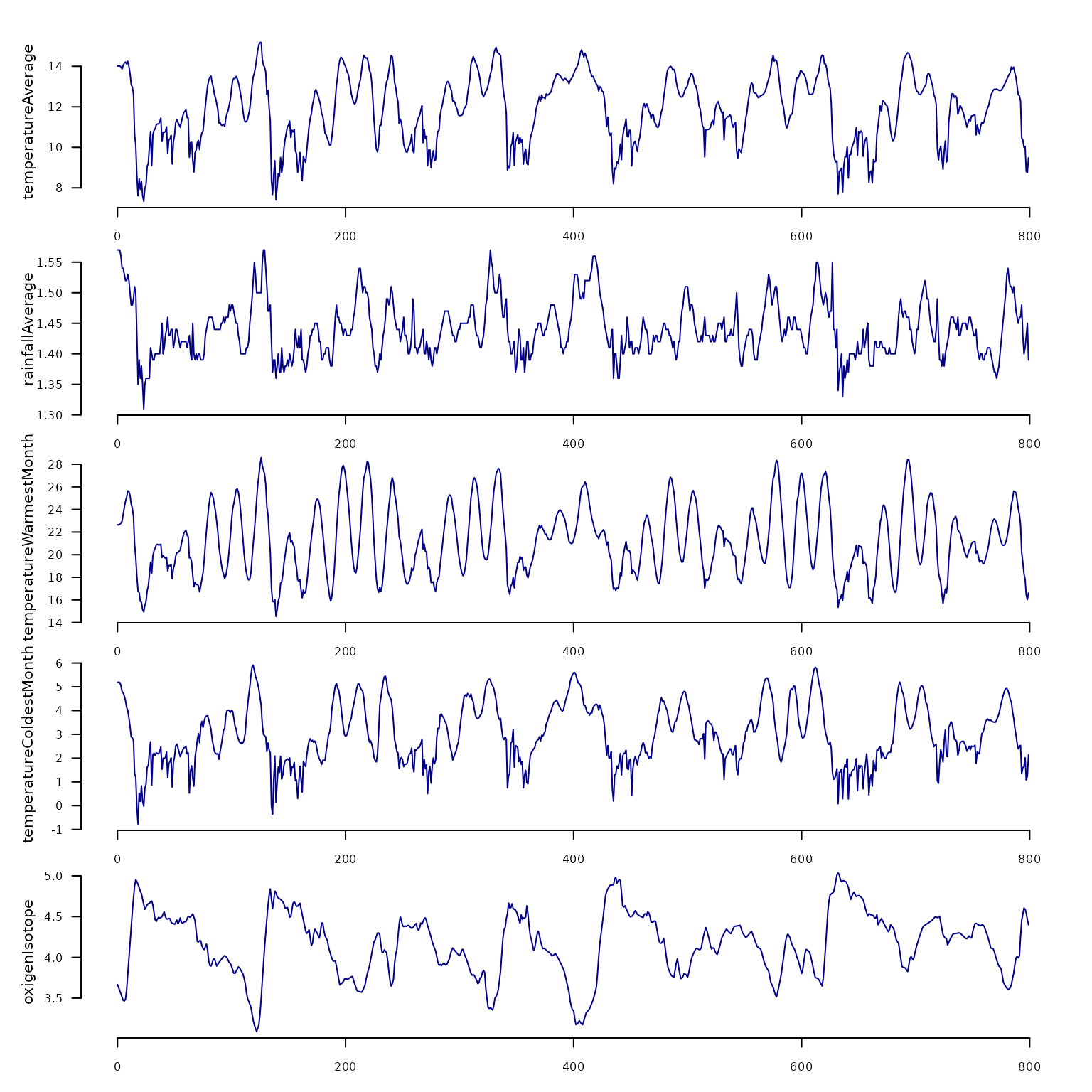
- climate: regular time series with 800 samples taken every 1000 years, with climate variables (temperature, rainfall, etc.)
data(climate, package = "memoria")

climate |>
  distantia::tsl_init(
    time_column = "age"
  ) |>
  distantia::tsl_plot(
    ylim = "relative",
    guide = FALSE,
    line_color = "blue4"
  )
Align Datasets
The package memoria requires the input time series to be
regular, but pollen is irregular, with a range of time
intervals between 0.32 and 6.475.
To homogenize both datasets, below we use linear interpolation with
time to align pollen with climate.
df <- memoria::alignTimeSeries(
  datasets.list = list(
    pollen = pollen,
    climate = climate
  ),
  time.column = "age",
  interpolation.interval = 1
)

nrow(df)
#> [1] 799
range(diff(df$age)) #1000 years
#> [1] 1 1
colnames(df)
#>  [1] "age"                             "pollen.pinus"
#>  [3] "pollen.quercus"                  "pollen.poaceae"
#>  [5] "pollen.artemisia"                "climate.temperatureAverage"
#>  [7] "climate.rainfallAverage"         "climate.temperatureWarmestMonth"
#>  [9] "climate.temperatureColdestMonth" "climate.oxigenIsotope"
Now that the responses and the drivers are at the same resolution, we just need to select the data we want to play with.
df <- df |>
  dplyr::transmute(
    time = age,
    quercus = pollen.quercus,
    rain = climate.rainfallAverage,
    temp = climate.temperatureAverage
  )
Create lagged data
The lagTimeSeries() function organizes data into the lag
structure required by the model. Each sample of the response is aligned
with antecedent values of itself and the drivers. In this case we use
lags 1 to 10, which correspond with 1000 to 10000 years.
quercus_lags <- lagTimeSeries(
  input.data = df,
  response = "quercus",
  drivers = c("rain", "temp"),
  time = "time",
  oldest.sample = "last",
  lags = seq(from = 1, to = 10, by = 1)
)
Note on oldest.sample: Set to
"last" when the oldest sample is at the bottom of the
dataframe (typical palaeoecological convention). Set to
"first" if the oldest sample is at the top.
The output columns follow a naming convention:
dplyr::glimpse(quercus_lags)
#> Rows: 789
#> Columns: 34
#> $ quercus__0  <dbl> 95.5869512, 134.9473077, 135.5032469, 102.7573460, 78.5362…
#> $ quercus__1  <dbl> 134.9473077, 135.5032469, 102.7573460, 78.5362180, 144.577…
#> $ quercus__2  <dbl> 135.5032469, 102.7573460, 78.5362180, 144.5770506, 130.868…
#> $ quercus__3  <dbl> 102.7573460, 78.5362180, 144.5770506, 130.8689767, 107.072…
#> $ quercus__4  <dbl> 78.5362180, 144.5770506, 130.8689767, 107.0723299, 84.5673…
#> $ quercus__5  <dbl> 144.5770506, 130.8689767, 107.0723299, 84.5673993, 59.7365…
#> $ quercus__6  <dbl> 130.8689767, 107.0723299, 84.5673993, 59.7365964, 82.09479…
#> $ quercus__7  <dbl> 107.0723299, 84.5673993, 59.7365964, 82.0947989, 37.212402…
#> $ quercus__8  <dbl> 84.5673993, 59.7365964, 82.0947989, 37.2124029, 0.0000000,…
#> $ quercus__9  <dbl> 59.7365964, 82.0947989, 37.2124029, 0.0000000, 0.0000000, …
#> $ quercus__10 <dbl> 82.0947989, 37.2124029, 0.0000000, 0.0000000, 1.0420467, 0…
#> $ rain__0     <dbl> 1.570000, 1.569424, 1.561583, 1.551496, 1.540789, 1.532796…
#> $ rain__1     <dbl> 1.569424, 1.561583, 1.551496, 1.540789, 1.532796, 1.525082…
#> $ rain__2     <dbl> 1.561583, 1.551496, 1.540789, 1.532796, 1.525082, 1.521579…
#> $ rain__3     <dbl> 1.551496, 1.540789, 1.532796, 1.525082, 1.521579, 1.524918…
#> $ rain__4     <dbl> 1.540789, 1.532796, 1.525082, 1.521579, 1.524918, 1.524046…
#> $ rain__5     <dbl> 1.532796, 1.525082, 1.521579, 1.524918, 1.524046, 1.509918…
#> $ rain__6     <dbl> 1.525082, 1.521579, 1.524918, 1.524046, 1.509918, 1.490164…
#> $ rain__7     <dbl> 1.521579, 1.524918, 1.524046, 1.509918, 1.490164, 1.479539…
#> $ rain__8     <dbl> 1.524918, 1.524046, 1.509918, 1.490164, 1.479539, 1.485871…
#> $ rain__9     <dbl> 1.524046, 1.509918, 1.490164, 1.479539, 1.485871, 1.503371…
#> $ rain__10    <dbl> 1.509918, 1.490164, 1.479539, 1.485871, 1.503371, 1.504261…
#> $ temp__0     <dbl> 14.082412, 14.003592, 13.963610, 13.962222, 13.994756, 14.…
#> $ temp__1     <dbl> 14.003592, 13.963610, 13.962222, 13.994756, 14.074843, 14.…
#> $ temp__2     <dbl> 13.963610, 13.962222, 13.994756, 14.074843, 14.159573, 14.…
#> $ temp__3     <dbl> 13.962222, 13.994756, 14.074843, 14.159573, 14.214738, 14.…
#> $ temp__4     <dbl> 13.994756, 14.074843, 14.159573, 14.214738, 14.203480, 14.…
#> $ temp__5     <dbl> 14.074843, 14.159573, 14.214738, 14.203480, 14.072493, 13.…
#> $ temp__6     <dbl> 14.159573, 14.214738, 14.203480, 14.072493, 13.798291, 13.…
#> $ temp__7     <dbl> 14.214738, 14.203480, 14.072493, 13.798291, 13.514943, 13.…
#> $ temp__8     <dbl> 14.203480, 14.072493, 13.798291, 13.514943, 13.153375, 12.…
#> $ temp__9     <dbl> 14.072493, 13.798291, 13.514943, 13.153375, 12.558464, 11.…
#> $ temp__10    <dbl> 13.798291, 13.514943, 13.153375, 12.558464, 11.686879, 10.…
#> $ time        <dbl> 0.5, 1.5, 2.5, 3.5, 4.5, 5.5, 6.5, 7.5, 8.5, 9.5, 10.5, 11…
quercus_lags |>
  dplyr::select(
    quercus__0,
    quercus__5,
    quercus__10,
    time
  ) |>
  dplyr::filter(
    time <= 100
  ) |>
  distantia::tsl_init(
    time_column = "time"
  ) |>
  distantia::tsl_plot()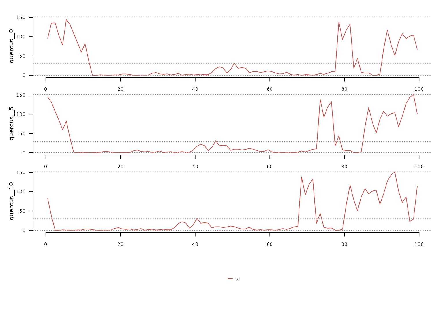
Ecological Memory Analysis
The computeMemory() function fits Random Forest models
on the lagged data. It measures variable importance using permutation,
which is robust to multicollinearity and temporal autocorrelation.
Two benchmark modes are available for significance testing:
-
"white.noise": Random values without temporal structure (faster) -
"autocorrelated": Random walk with temporal structure (more conservative, recommended)
The model runs multiple times (repetitions),
regenerating the random term each time, then computes percentiles of
importance scores.
quercus_memory <- memoria::computeMemory(
  lagged.data = quercus_lags,
  random.mode = "autocorrelated",
  repetitions = 100
)
We can visualize the results with plotMemory().
memoria::plotMemory(quercus_memory)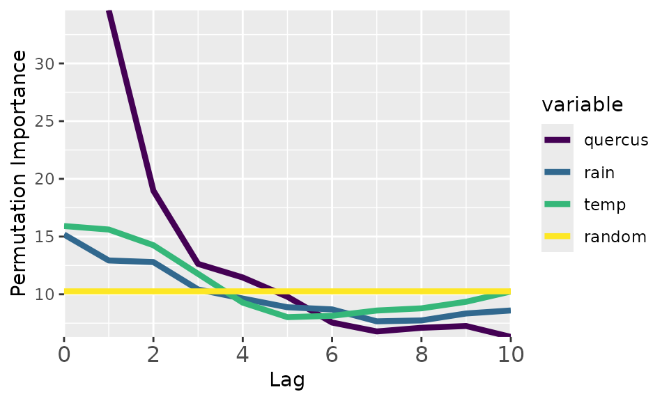
The plot shows all ecological memory components of this dataset.
Endogenous memory (“quercus” curve): shows the importance of the past pollen abundance in predicting current pollen abundance. In this case, this is the most important memory component, with a lag of ~5000 years.
Significance test (“random” curve): shows the median importance scores of randomly generated variables. Defines a baseline helpful to know when a given memory component explains the response better (above the yellow line) or worse than random.
Concurrent effect (“temp” and “rain” at lag 0): importance of the current driver values to predict the response. In this case, the concurrent effect is much weaker than the endogenous memory.
Exogenous memory (“temp” and “rain” at lag > 0): importance of the past driver values in explaining the current response values. According to the plot, temperature is the strongest component of the exogenous memory, with a lag of almost ~4000 years.
The extractMemoryFeatures() function transforms the plot
results into quantitative features:
extractMemoryFeatures(
  memory.pattern = quercus_memory
) |>
  dplyr::glimpse()
#> Rows: 1
#> Columns: 8
#> $ label                <chr> "quercus"
#> $ strength.endogenous  <dbl> 24.35066
#> $ strength.exogenous   <dbl> 5.351078
#> $ strength.concurrent  <dbl> 5.653404
#> $ length.endogenous    <dbl> 0.4
#> $ length.exogenous     <dbl> 0.3
#> $ dominance.endogenous <dbl> 0.4
#> $ dominance.exogenous  <dbl> 0
The output contains eight features organized in three groups:
The strength values (scaled to [0, 1] by default) measure the peak importance of each memory component relative to the median of the random baseline.
The length values (proportion in [0, 1]) measure how far into the past each memory component remains above the random baseline. In this case, the endogenous memory component is above the baseline for half of the lags.
The dominance values (proportion in [0, 1]) measure whether endogenous or exogenous memory prevails across significant lags. In this case, the exogenous memory is never above the endogenous one, hence it has zero dominance.
Summary
The complete workflow:
-
alignTimeSeries()- Align datasets with different resolutions. -
lagTimeSeries()- Create lag structure. -
computeMemory()- Fit Random Forest and compute importance. -
plotMemory()- Visualize the memory pattern. -
extractMemoryFeatures()- Quantify memory characteristics.