memoria and virtualPollen

Introduction

The virtualPollen package generates synthetic pollen abundance curves by simulating virtual taxa with configurable life-history traits (maximum age, fecundity) and niche characteristics (optimum, breadth). Combined with memoria, this creates a powerful framework for systematically exploring how species traits modulate ecological memory patterns.

This article demonstrates how to run batch memory analyses across multiple virtual taxa using memoria’s experiment functions. For methodological details, see:

Benito, B.M., Gil-Romera, G. and Birks, H.J.B. (2020). Ecological memory at millennial time-scales: the importance of data constraints, species longevity and niche features. Ecography, 43: 1-10. https://doi.org/10.1111/ecog.04772

Setup

library(memoria)
library(virtualPollen)
library(ggplot2)
library(dplyr)

The virtualPollen Package

virtualPollen simulates pollen abundance curves using a population dynamics model where virtual taxa have configurable traits (life-span, fecundity, growth rate), environmental drivers influence population dynamics through species-specific response functions, and niche parameters define how each taxon responds to environmental gradients.

Key trait parameters and their expected effects on memory:

Parameter	Description	Expected Memory Effect
`maximum.age`	Maximum lifespan of individuals	Longer life → extended endogenous memory
`fecundity`	Number of offspring per reproductive event	Affects population recovery dynamics
`niche.A.sd`	Niche breadth (standard deviation)	Broader niche → weaker exogenous memory
`niche.A.mean`	Niche optimum position	Determines driver response curve

Understanding the Data

The virtualPollen package provides two example datasets: parameters and simulation.

The virtualPollen::parameters dataframe describes the traits of the simulated species. Note the contrast between short-lived (maximum.age = 10) and long-lived (maximum.age = 1000) taxa, and between high (fecundity = 10) and low (fecundity = 1) fecundity.

data(parameters, package = "virtualPollen")
dplyr::glimpse(parameters)
#> Rows: 4
#> Columns: 16
#> $ label                    <chr> "S10A50-5_f10", "S1000A50-5_f10", "S10A50-5_f…
#> $ maximum.age              <dbl> 10, 1000, 10, 1000
#> $ reproductive.age         <dbl> 4, 100, 4, 100
#> $ fecundity                <dbl> 10, 10, 1, 1
#> $ growth.rate              <dbl> 1.50, 0.01, 1.50, 0.01
#> $ pollen.control           <dbl> 0, 0, 0, 0
#> $ maximum.biomass          <dbl> 100, 100, 100, 100
#> $ carrying.capacity        <dbl> 10000, 10000, 10000, 10000
#> $ driver.A.weight          <dbl> 1, 1, 1, 1
#> $ driver.B.weight          <dbl> 0, 0, 0, 0
#> $ niche.A.mean             <dbl> 50, 50, 50, 50
#> $ niche.A.sd               <dbl> 10, 10, 10, 10
#> $ niche.B.mean             <dbl> 50, 50, 50, 50
#> $ niche.B.sd               <dbl> 5, 5, 5, 5
#> $ autocorrelation.length.A <dbl> 600, 600, 600, 600
#> $ autocorrelation.length.B <dbl> 600, 600, 600, 600

The virtualPollen::simulation dataset is a list containing simulated populations generated by virtualPollen::simulatePopulation() using parameters as input.

data(simulation, package = "virtualPollen")
str(simulation, max.level = 1)
#> List of 4
#>  $ S10A50-5_f10  :'data.frame':  5000 obs. of  14 variables:
#>  $ S1000A50-5_f10:'data.frame':  5000 obs. of  14 variables:
#>  $ S10A50-5_f1   :'data.frame':  5000 obs. of  14 variables:
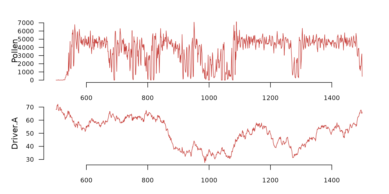
#>  $ S1000A50-5_f1 :'data.frame':  5000 obs. of  14 variables:

Each element is a dataframe with the results of a mechanistic simulation. The plot below shows a small section and subset of variables from the first simulated time series.

Batch Memory Analysis with `memoria::runExperiment()`

The runExperiment() function applies the full memoria workflow across multiple virtual taxa and sampling resolutions:

experiment <- memoria::runExperiment(
  simulations.file = simulation,
  parameters.file = parameters,
  parameters.names = c(
    "maximum.age",
    "fecundity"
  ),
  driver.column = "Driver.A",
  response.column = "Pollen",
  time.column = "Time",
  lags = seq(10, 120, by = 10),
  repetitions = 30
)

Visualizing Results with plotExperiment()

The plotExperiment() function generates faceted plots showing memory patterns across all analyzed taxa:

memoria::plotExperiment(
  experiment.output = experiment,
  parameters.file = parameters
)

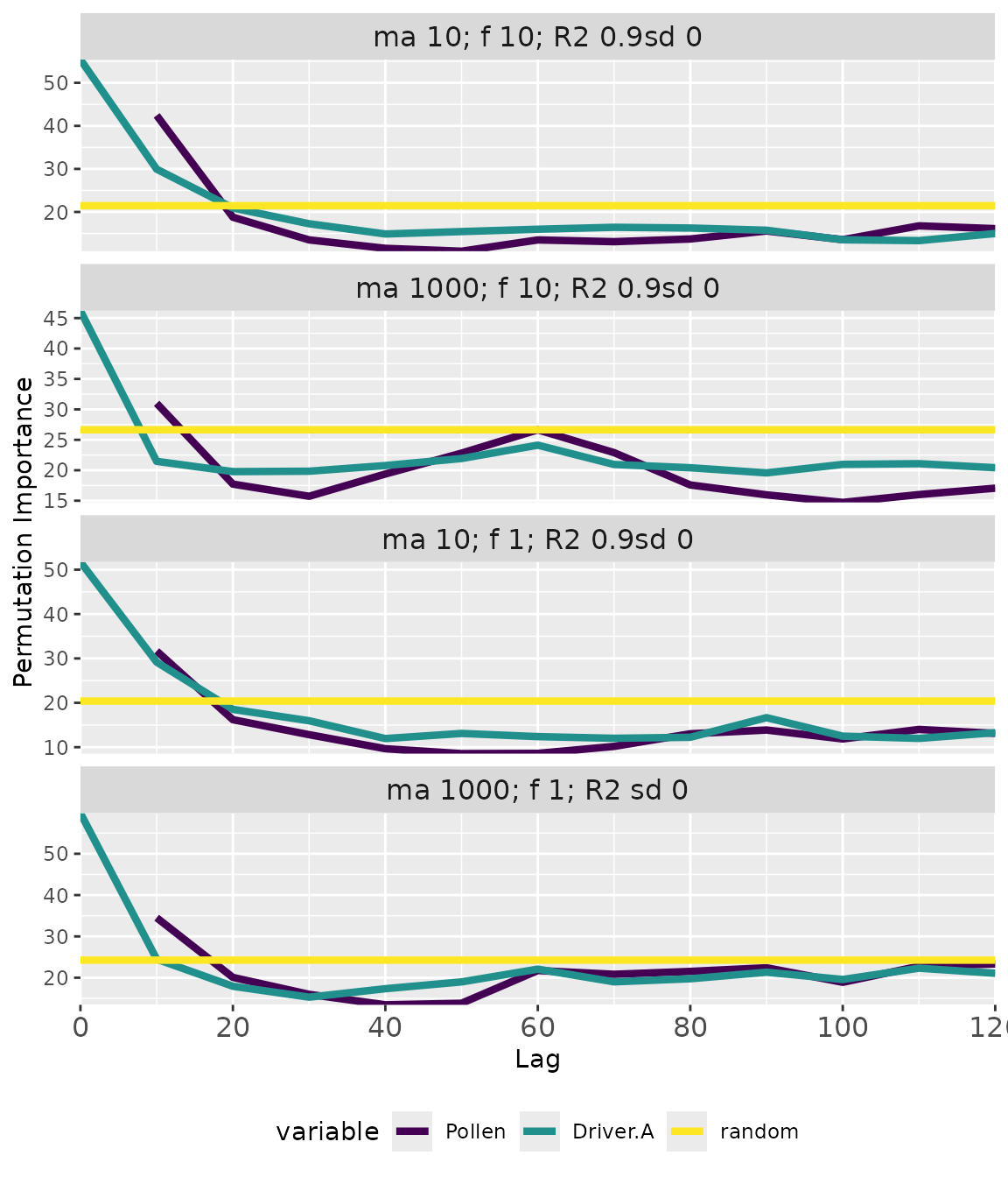
Interpreting the plot:

Lines: Median importance across repetitions.
Ribbons: 5th-95th percentile confidence intervals.
Facets: Each panel shows a different taxon with its trait values.
Colors: Different memory components (response = endogenous, driver = exogenous, random = significance baseline).
R2 values: Model fit (pseudo R-squared from Random Forest).

When importance exceeds the random baseline, that memory component explains variation in pollen abundance better than chance.

Converting to Table Format

The experimentToTable() function reshapes experiment results into a long-format dataframe for further analysis:

experiment_table <- experimentToTable(
  experiment.output = experiment,
  parameters.file = virtualPollen::parameters
)

dplyr::glimpse(experiment_table)
#> Rows: 152
#> Columns: 25
#> $ median                   <dbl> 42.43117, 18.77682, 13.50895, 11.55201, 10.88…
#> $ sd                       <dbl> 1.0158766, 0.6630606, 0.7150361, 0.7762626, 1…
#> $ min                      <dbl> 40.455338, 17.560109, 12.484472, 10.463731, 9…
#> $ max                      <dbl> 44.07475, 19.33819, 14.63643, 12.67534, 12.78…
#> $ variable                 <fct> Pollen, Pollen, Pollen, Pollen, Pollen, Polle…
#> $ lag                      <dbl> 10, 20, 30, 40, 50, 60, 70, 80, 90, 100, 110,…
#> $ name                     <chr> "ma 10; f 10; R2 0.9sd 0", "ma 10; f 10; R2 0…
#> $ R2mean                   <dbl> 0.9797754, 0.9797754, 0.9797754, 0.9797754, 0…
#> $ R2sd                     <dbl> 0.00010613, 0.00010613, 0.00010613, 0.0001061…
#> $ label                    <chr> "S10A50-5_f10", "S10A50-5_f10", "S10A50-5_f10…
#> $ maximum.age              <dbl> 10, 10, 10, 10, 10, 10, 10, 10, 10, 10, 10, 1…
#> $ reproductive.age         <dbl> 4, 4, 4, 4, 4, 4, 4, 4, 4, 4, 4, 4, 4, 4, 4, …
#> $ fecundity                <dbl> 10, 10, 10, 10, 10, 10, 10, 10, 10, 10, 10, 1…
#> $ growth.rate              <dbl> 1.5, 1.5, 1.5, 1.5, 1.5, 1.5, 1.5, 1.5, 1.5, …
#> $ pollen.control           <dbl> 0, 0, 0, 0, 0, 0, 0, 0, 0, 0, 0, 0, 0, 0, 0, …
#> $ maximum.biomass          <dbl> 100, 100, 100, 100, 100, 100, 100, 100, 100, …
#> $ carrying.capacity        <dbl> 10000, 10000, 10000, 10000, 10000, 10000, 100…
#> $ driver.A.weight          <dbl> 1, 1, 1, 1, 1, 1, 1, 1, 1, 1, 1, 1, 1, 1, 1, …
#> $ driver.B.weight          <dbl> 0, 0, 0, 0, 0, 0, 0, 0, 0, 0, 0, 0, 0, 0, 0, …
#> $ niche.A.mean             <dbl> 50, 50, 50, 50, 50, 50, 50, 50, 50, 50, 50, 5…
#> $ niche.A.sd               <dbl> 10, 10, 10, 10, 10, 10, 10, 10, 10, 10, 10, 1…
#> $ niche.B.mean             <dbl> 50, 50, 50, 50, 50, 50, 50, 50, 50, 50, 50, 5…
#> $ niche.B.sd               <dbl> 5, 5, 5, 5, 5, 5, 5, 5, 5, 5, 5, 5, 5, 5, 5, …
#> $ autocorrelation.length.A <dbl> 600, 600, 600, 600, 600, 600, 600, 600, 600, …
#> $ autocorrelation.length.B <dbl> 600, 600, 600, 600, 600, 600, 600, 600, 600, …

The output includes:

Variable, Lag: Memory component and time lag.
median, min, max: Importance statistics across repetitions.
R2mean, R2sd: Model fit statistics.

Extracting Memory Features

The extractMemoryFeatures() function can process output from experimentToTable() to compute the eight memory features for each taxon:

features <- memoria::extractMemoryFeatures(
  memory.pattern = experiment_table,
  exogenous.component = "Driver.A",
  endogenous.component = "Pollen"
)

dplyr::glimpse(features)
#> Rows: 4
#> Columns: 12
#> $ label                <chr> "S10A50-5_f10", "S1000A50-5_f10", "S10A50-5_f1", …
#> $ strength.endogenous  <dbl> 1.0000000, 0.2075139, 0.5378882, 0.4891335
#> $ strength.exogenous   <dbl> 0.96585579, 0.00000000, 1.00000000, 0.02699637
#> $ strength.concurrent  <dbl> 0.9544150, 0.5498155, 0.8813975, 1.0000000
#> $ length.endogenous    <dbl> 0.08333333, 0.08333333, 0.08333333, 0.08333333
#> $ length.exogenous     <dbl> 0.08333333, 0.00000000, 0.08333333, 0.08333333
#> $ dominance.endogenous <dbl> 0.08333333, 0.08333333, 0.08333333, 0.08333333
#> $ dominance.exogenous  <dbl> 0, 0, 0, 0
#> $ maximum.age          <dbl> 10, 1000, 10, 1000
#> $ fecundity            <dbl> 10, 10, 1, 1
#> $ niche.mean           <dbl> 50, 50, 50, 50
#> $ niche.sd             <dbl> 10, 10, 10, 10

The eight features (organized in three groups):

Strength (scaled 0-1): Peak importance relative to random baseline.

strength.endogenous: How strongly past pollen predicts current pollen.
strength.exogenous: How strongly past environment predicts current pollen.
strength.concurrent: How strongly current environment predicts current pollen.

Length (proportion 0-1): How far into the past memory extends above baseline.

length.endogenous: Temporal extent of significant endogenous memory.
length.exogenous: Temporal extent of significant exogenous memory.

Dominance (proportion 0-1): Which component prevails across significant lags.

dominance.endogenous: Proportion of lags where endogenous > exogenous.
dominance.exogenous: Proportion of lags where exogenous > endogenous.

Summary

The integration of virtualPollen and memoria enables systematic exploration of ecological memory:

virtualPollen generates synthetic pollen curves with known trait parameters.
runExperiment() applies the memoria workflow across multiple taxa/resolutions.
plotExperiment() visualizes memory patterns in faceted plots.
experimentToTable() converts results to analyzable long format.
extractMemoryFeatures() quantifies the eight memory features.

This framework revealed that life-span and niche features fundamentally shape ecological memory patterns, with important implications for interpreting palaeoecological records and climate reconstructions.

For complete methodological details and extended analysis, see:

Benito, B.M., Gil-Romera, G. and Birks, H.J.B. (2020). Ecological memory at millennial time-scales: the importance of data constraints, species longevity and niche features. Ecography, 43: 1-10. https://doi.org/10.1111/ecog.04772