Working with memoria • memoria

This article walks through the complete memoria workflow for quantifying ecological memory in time series data consisting of at least one response and one predictor.

Ecological Memory

The package memoria helps quantify how past and concurrent events shape the state of a system. This concept is summarized in the figure below:

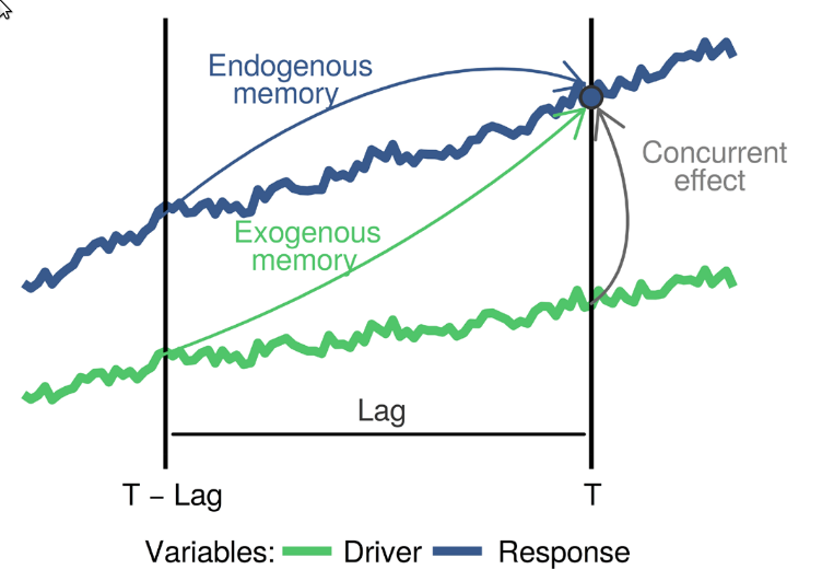Ecological Memory The blue and green curves represent the values of a biotic response y and a driver x over time. The vertical line T represents the current time, while T - lag represents a a previous time. The arrows represent influence, as follows:

Endogenous memory: is the effect of past y on present y.
Exogenous memory: is the effect of past x on present y.
Concurrent effect: is the effect of present x on present y.

To assess these effects, memoria generates the lagged data and trains the model

$y_{T} = y_{T-1} + \ldots + y_{T-n} + x_{T} + x_{T-1} + \ldots + x_{T-n} + r_{T}$

Where:

$y$ and $x$ are the response and the driver.
$T$ is the “current” time, and $t-1$ to $t-n$ , are the time lags.
$y_{T-1} + \ldots + y_{T-n}$ represents the endogenous memory across lags.
$x_{T-1} + \ldots + x_{T-n}$ represents the exogenous memory across lags.
$x_{T}$ represents the concurrent effect.
$r_{T}$ is a random term used to assess statistical significance.

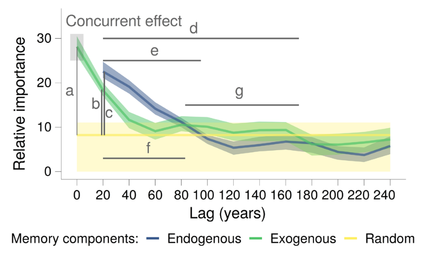
The ecological memory pattern is quantified using permutation importance from Random Forest models. For each predictor, the algorithm shuffles its values and measures the decrease in predictive accuracy—larger decreases indicate stronger influence on the response.

Ecological Memory

The following sections demonstrate how to implement this workflow in R using the memoria package.

Setup

library(memoria)
library(ggplot2)
library(tidyr)
library(knitr)

Workflow

Merge datasets

The mergePalaeoData() function aligns and interpolates datasets sampled at different resolutions. Consider two built-in datasets:

pollen: 639 samples with four pollen types (Pinus, Quercus, Poaceae, Artemisia)
climate: 800 samples with climate variables (temperature, rainfall, etc.)

data(pollen)

ggplot(
  data = gather(pollen, pollen.type, pollen.abundance, 2:5),
  aes(x = age, y = pollen.abundance, group = pollen.type)
) +
  geom_line() +
  facet_wrap(vars(pollen.type), ncol = 1, scales = "free_y") +
  xlab("Age (ky BP)") +
  ylab("Pollen counts") +
  ggtitle("Pollen dataset")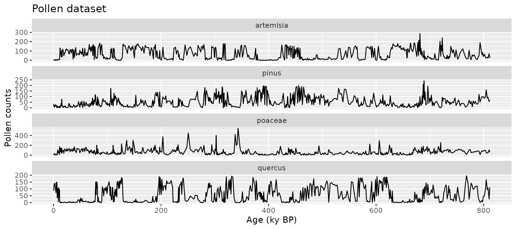

data(climate)

ggplot(
  data = gather(climate, variable, value, 2:5),
  aes(x = age, y = value, group = variable)
) +
  geom_line() +
  facet_wrap(vars(variable), ncol = 1, scales = "free_y") +
  xlab("Age (ky BP)") +
  ylab("") +
  ggtitle("Palaeoclimatic data")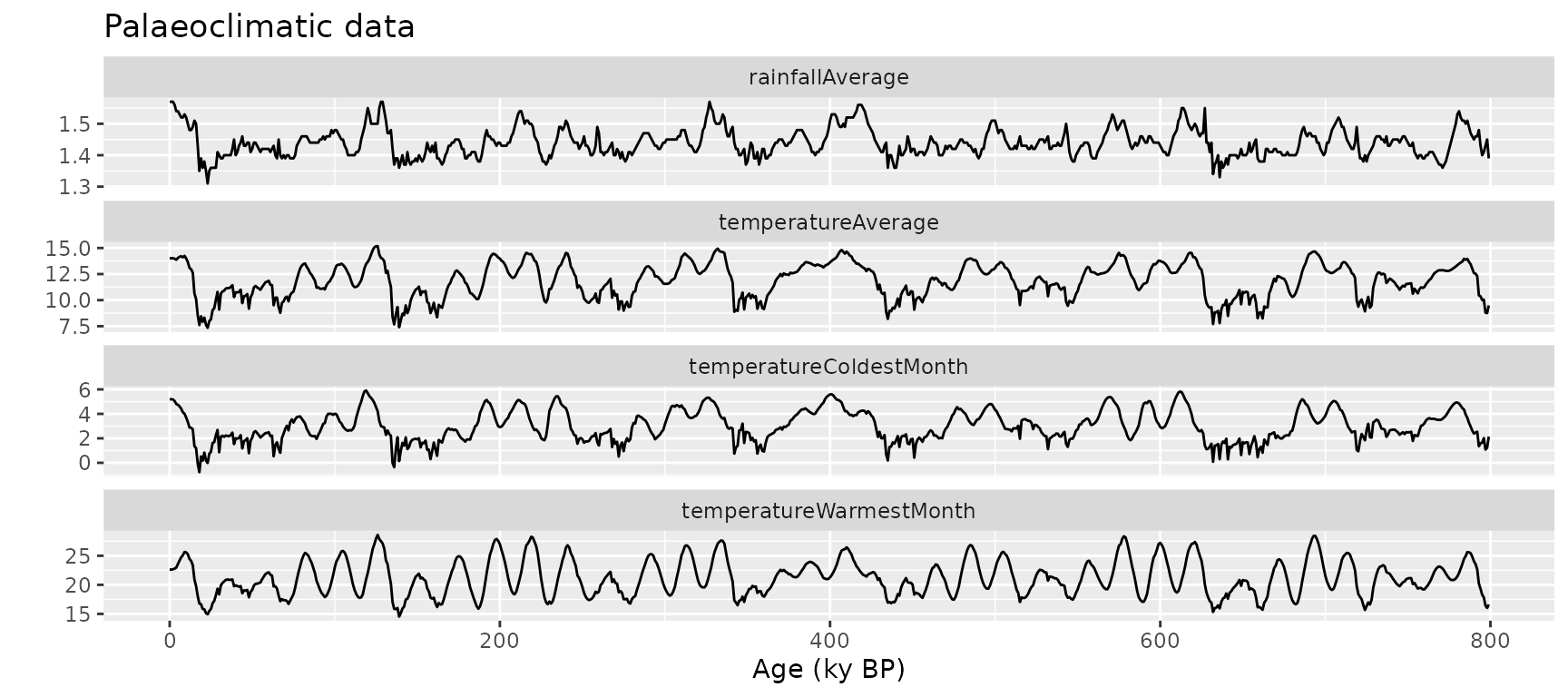

Merge and interpolate into a regular time grid:

pollen_climate <- mergePalaeoData(
  datasets.list = list(
    pollen = pollen,
    climate = climate
  ),
  time.column = "age",
  interpolation.interval = 0.2
)
#> Argument interpolation.interval is set to 0.2
#> The average temporal resolution of pollen is 1.27; you are incrementing data resolution by a factor of 6.35
#> The average temporal resolution of climate is 1; you are incrementing data resolution by a factor of 5

str(pollen_climate)
#> 'data.frame':    3993 obs. of  10 variables:
#>  $ age                            : num  0.5 0.7 0.9 1.1 1.3 1.5 1.7 1.9 2.1 2.3 ...
#>  $ pollen.pinus                   : num  0 2.5 6.97 10.64 13.39 ...
#>  $ pollen.quercus                 : num  95.6 109.4 120.1 127.7 132.6 ...
#>  $ pollen.poaceae                 : num  0 9.55 16.79 21.76 24.76 ...
#>  $ pollen.artemisia               : num  0 0 0.672 1.696 2.516 ...
#>  $ climate.temperatureAverage     : num  14.1 14.1 14 14 14 ...
#>  $ climate.rainfallAverage        : num  1.57 1.57 1.57 1.57 1.57 ...
#>  $ climate.temperatureWarmestMonth: num  21 21.3 21.5 21.7 21.8 ...
#>  $ climate.temperatureColdestMonth: num  5.25 5.24 5.23 5.22 5.2 ...
#>  $ climate.oxigenIsotope          : num  3.43 3.43 3.43 3.44 3.44 ...

ggplot(
  data = gather(pollen_climate, variable, value, 2:10),
  aes(x = age, y = value, group = variable)
) +
  geom_line() +
  facet_wrap(vars(variable), ncol = 1, scales = "free_y") +
  xlab("Age (ky BP)") +
  ylab("") +
  ggtitle("Pollen and palaeoclimate (merged)")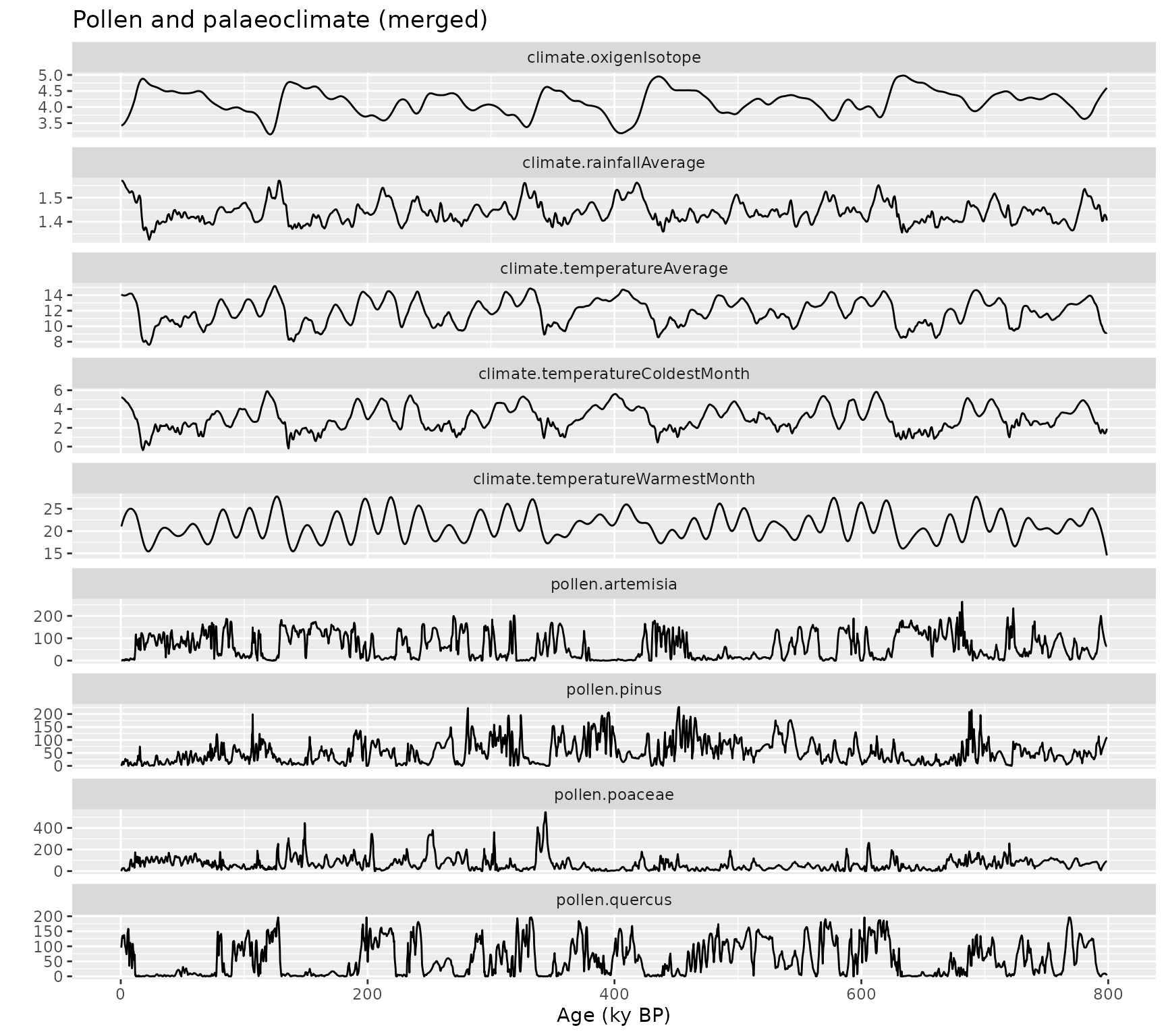

Create lagged data

The prepareLaggedData() function organizes data into the lag structure required by the model. Each sample of the response is aligned with antecedent values of itself and the drivers.

pollen_climate_lagged <- prepareLaggedData(
  input.data = pollen_climate,
  response = "pollen.pinus",
  drivers = c("climate.temperatureAverage", "climate.rainfallAverage"),
  time = "age",
  oldest.sample = "last",
  lags = seq(0.2, 1, by = 0.2)
)

str(pollen_climate_lagged)
#> 'data.frame':    3988 obs. of  19 variables:
#>  $ pollen.pinus__0                : num  0 2.5 6.97 10.64 13.39 ...
#>  $ pollen.pinus__0.2              : num  2.5 6.97 10.64 13.39 15.02 ...
#>  $ pollen.pinus__0.4              : num  6.97 10.64 13.39 15.02 15.62 ...
#>  $ pollen.pinus__0.6              : num  10.6 13.4 15 15.6 14.5 ...
#>  $ pollen.pinus__0.8              : num  13.4 15 15.6 14.5 10.9 ...
#>  $ pollen.pinus__1                : num  15 15.6 14.5 10.9 6 ...
#>  $ climate.temperatureAverage__0  : num  14.1 14.1 14 14 14 ...
#>  $ climate.temperatureAverage__0.2: num  14.1 14 14 14 14 ...
#>  $ climate.temperatureAverage__0.4: num  14 14 14 14 14 ...
#>  $ climate.temperatureAverage__0.6: num  14 14 14 14 14 ...
#>  $ climate.temperatureAverage__0.8: num  14 14 14 14 14 ...
#>  $ climate.temperatureAverage__1  : num  14 14 14 14 14 ...
#>  $ climate.rainfallAverage__0     : num  1.57 1.57 1.57 1.57 1.57 ...
#>  $ climate.rainfallAverage__0.2   : num  1.57 1.57 1.57 1.57 1.57 ...
#>  $ climate.rainfallAverage__0.4   : num  1.57 1.57 1.57 1.57 1.57 ...
#>  $ climate.rainfallAverage__0.6   : num  1.57 1.57 1.57 1.57 1.57 ...
#>  $ climate.rainfallAverage__0.8   : num  1.57 1.57 1.57 1.57 1.56 ...
#>  $ climate.rainfallAverage__1     : num  1.57 1.57 1.57 1.56 1.56 ...
#>  $ time                           : num  0.5 0.7 0.9 1.1 1.3 1.5 1.7 1.9 2.1 2.3 ...
#>  - attr(*, "response")= chr "pollen.pinus"
#>  - attr(*, "drivers")= chr [1:2] "climate.temperatureAverage" "climate.rainfallAverage"

# Check attributes (used by computeMemory for auto-detection)
attr(pollen_climate_lagged, "response")
#> [1] "pollen.pinus"
attr(pollen_climate_lagged, "drivers")
#> [1] "climate.temperatureAverage" "climate.rainfallAverage"

Note on oldest.sample: Set to "last" when the oldest sample is at the bottom of the dataframe (typical palaeoecological convention). Set to "first" if the oldest sample is at the top.

The output columns follow a naming convention:

pollen.pinus__0: Current response value
pollen.pinus__0.2, pollen.pinus__0.4, etc.: Endogenous terms
climate.temperatureAverage__0, climate.temperatureAverage__0.2, etc.: Concurrent effect and exogenous terms

Compute memory

The computeMemory() function fits Random Forest models on the lagged data. It measures variable importance using permutation, which is robust to multicollinearity and temporal autocorrelation.

Two benchmark modes are available for significance testing:

"white.noise": Random values without temporal structure (faster)
"autocorrelated": Random walk with temporal structure (more conservative, recommended)

The model runs multiple times (repetitions), regenerating the random term each time, then computes percentiles of importance scores.

# Simplified call - response and drivers auto-detected from lagged data attributes
memory_output <- computeMemory(
  lagged.data = pollen_climate_lagged,
  random.mode = "white.noise",
  repetitions = 100
)

# Output structure (5 slots)
names(memory_output)
#> [1] "response"   "drivers"    "memory"     "R2"         "prediction"

# Memory dataframe (lowercase column names: variable, lag)
head(memory_output$memory)
#>     median        sd      min      max                   variable lag
#> 1 40.68684 1.0008733 39.36679 42.42693               pollen.pinus 0.2
#> 2 25.25720 0.7842455 24.07659 26.52628               pollen.pinus 0.4
#> 3 17.18441 0.9590776 15.63918 18.74209               pollen.pinus 0.6
#> 4 15.57412 1.4198263 13.37104 18.24264               pollen.pinus 0.8
#> 5 18.78565 1.0239717 16.99415 20.41879               pollen.pinus 1.0
#> 6 18.53973 1.8083562 15.58879 21.22939 climate.temperatureAverage 0.0

# Pseudo R-squared
head(memory_output$R2)
#> [1] 0.9910341 0.9910674 0.9909211 0.9908772 0.9909376 0.9908922

# Plot
plotMemory(memory_output)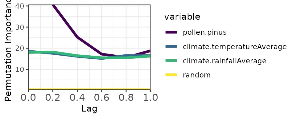

Now with autocorrelated random mode (more stringent):

memory_output_autocor <- computeMemory(
  lagged.data = pollen_climate_lagged,
  random.mode = "autocorrelated",
  repetitions = 100
)

plotMemory(memory_output_autocor)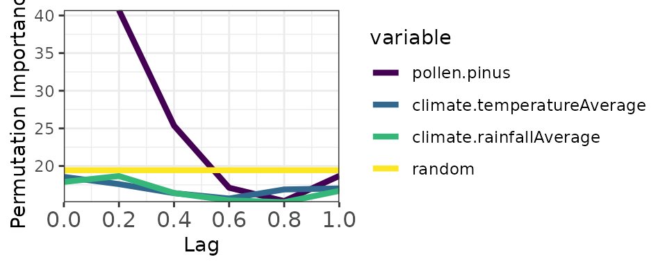

Notice the yellow band (random benchmark) is higher with autocorrelated mode, providing a more conservative significance threshold.

Extract memory features

The extractMemoryFeatures() function summarizes memory patterns into quantitative features:

memory_features <- extractMemoryFeatures(
  memory.pattern = memory_output_autocor,
  exogenous.component = c(
    "climate.temperatureAverage",
    "climate.rainfallAverage"
  ),
  endogenous.component = "pollen.pinus",
  sampling.subset = NULL,
  scale.strength = TRUE
)

kable(memory_features)

label	strength.endogenous	strength.exogenous	strength.concurrent	length.endogenous	length.exogenous	dominance.endogenous	dominance.exogenous
1	21.27227	0	-0.8896378	0.4	0	0.4	0

Understanding the Output

Significance testing

Random Forest provides importance scores but no built-in significance test. The solution is to add a random benchmark variable: if a predictor’s importance equals or falls below the random variable’s importance, we cannot distinguish its contribution from noise.

In plots, predictors with importance above the yellow band (random median) are considered significant. The width of the band reflects uncertainty across model repetitions.

The autocorrelated benchmark is recommended for palaeoecological analysis because it accounts for the temporal structure inherent in these datasets.

Memory features

The extracted features quantify three aspects of ecological memory:

Strength: Maximum importance difference between a component and the random median. Higher values indicate stronger memory effects. Computed for endogenous, exogenous, and concurrent components.
Length: Proportion of lags where importance exceeds the random median. Values near 1 indicate persistent memory across all lags. Computed for endogenous and exogenous components only.
Dominance: Among significant lags, the proportion where one component (endogenous or exogenous) exceeds the other. Values near 1 indicate one component dominates; values near 0.5 indicate balance.

Batch Experiments

The memoria package includes functions for batch analysis of simulated pollen curves from the virtualPollen package:

runExperiment(): Apply the full workflow across multiple simulations
experimentToTable(): Reshape experiment results into long format
plotExperiment(): Visualize memory patterns across parameter combinations

These functions enable systematic exploration of how ecological memory varies with species traits and sampling resolution. The virtualPollen package must be installed separately from GitHub (devtools::install_github("BlasBenito/virtualPollen")).

Summary

The complete workflow:

mergePalaeoData() - Align datasets with different resolutions
prepareLaggedData() - Create lag structure
computeMemory() - Fit Random Forest and compute importance
plotMemory() - Visualize the memory pattern
extractMemoryFeatures() - Quantify memory characteristics