Unified Correlation Framework

Summary

The function cor_df() combines several methods to compute pairwise associations between variables of different types:

• Numeric vs. numeric: Pearson correlation.
• Numeric vs. categorical: Combines target encoding and Pearson correlation.
• Categorical vs. categorical: Bias-corrected Cramer’s V.

This article provides fine-grained details on this functionality and describes the caveats of combining Pearson correlation and Cramer’s V when the cardinality of categorical predictors is high.

Setup

This article requires the following setup Don’t miss the object predictors and the variables it contains, as most of the explanatory code herein will be focusing on these.

Understanding cor_df()

This section explains in detail how cor_df() handles the computation of associations between different variable types.

When we apply cor_df() to a dataframe and a vector of predictors, it returns a dataframe with the Pearson or Cramer’s V association between all unique pairs of predictors.

x <- collinear::cor_df(
  df = vi_smol,
  predictors = predictors,
  quiet = TRUE
)

x
#>                  x             y correlation     metric
#> 1 temperature_mean   koppen_zone   0.9283292    Pearson
#> 2    rainfall_mean   koppen_zone   0.8443112    Pearson
#> 3    rainfall_mean     soil_type   0.6741559    Pearson
#> 4 temperature_mean     soil_type   0.6406734    Pearson
#> 5      koppen_zone     soil_type   0.3146128 Cramer's V
#> 6 temperature_mean rainfall_mean   0.2126887    Pearson

Let’s examine how the function handles different predictor types.

Numeric vs. Numeric

This is the simplest and most reliable case cor_df() handles, as pairwise Pearson correlations are computed with the very fast stats::cor().

The parallelization setup is ignored in this case.

predictors_numeric <- collinear::identify_numeric_variables(
  df = vi_smol,
  predictors = predictors
)$valid

stats::cor(
  x = vi_smol[, predictors_numeric],
  use = "complete.obs",
  method = "pearson"
) |> 
  abs()
#>                  temperature_mean rainfall_mean
#> temperature_mean        1.0000000     0.2126887
#> rainfall_mean           0.2126887     1.0000000

Numeric vs. Categorical

To handle this situation, cor_df() first applies target encoding to the categorical predictor using the numeric variable as reference, then applies stats::cor() to compute the Pearson correlation.

#transform koppen_zone to numeric
df <- target_encoding_lab(
  df = vi_smol,
  response = "temperature_mean",
  predictors = "koppen_zone",
  encoding_method = "loo",
  overwrite = TRUE,
  quiet = TRUE
)

stats::cor(
  x = df[["temperature_mean"]],
  y = df[["koppen_zone"]],
  use = "complete.obs",
  method = "pearson"
) |>
  abs()
#> [1] 0.9283292

Categorical vs. Categorical

This case is solved via bias-corrected Cramer’s V, based on Pearson’s chi-squared statistic. This method is implemented in the function cor_cramer().

collinear::cor_cramer(
  x = vi_smol[["koppen_zone"]],
  y = vi_smol[["soil_type"]]
)
#> [1] 0.3146128

Comparing Cramer’s V and Pearson Correlation

Now that you know how cor_df() handles different cases, there is an important question to answer: Are Cramer’s V and Pearson correlation comparable?

Let’s try to answer that question empirically with a small simulation. It generates integer vectors with different cardinality levels and compares them using both stats::cor() and cor_cramer().

set.seed(1)

#simulation parameters
sim <- data.frame(
  classes = rep(x = c(2, 4, 8, 16), times = 1000),
  cor = NA_real_,
  cramer_v = NA_real_
)

#run simulation
for(i in seq_len(nrow(sim))) {
  
  #generate integer vector with n classes
  x <- sample(x = 1:sim$classes[i], size = 30, replace = TRUE)
  
  #reshuffle x to get y with same marginal distribution
  y <- sample(x)
  
  #compute absolute Pearson correlation
  sim$cor[i] <- abs(stats::cor(x, y))
  
  #compute Cramer's V
  sim$cramer_v[i] <- collinear::cor_cramer(x, y)
  
}

The scatterplot below shows the simulation results across cardinality levels, with linear smooths for each group.

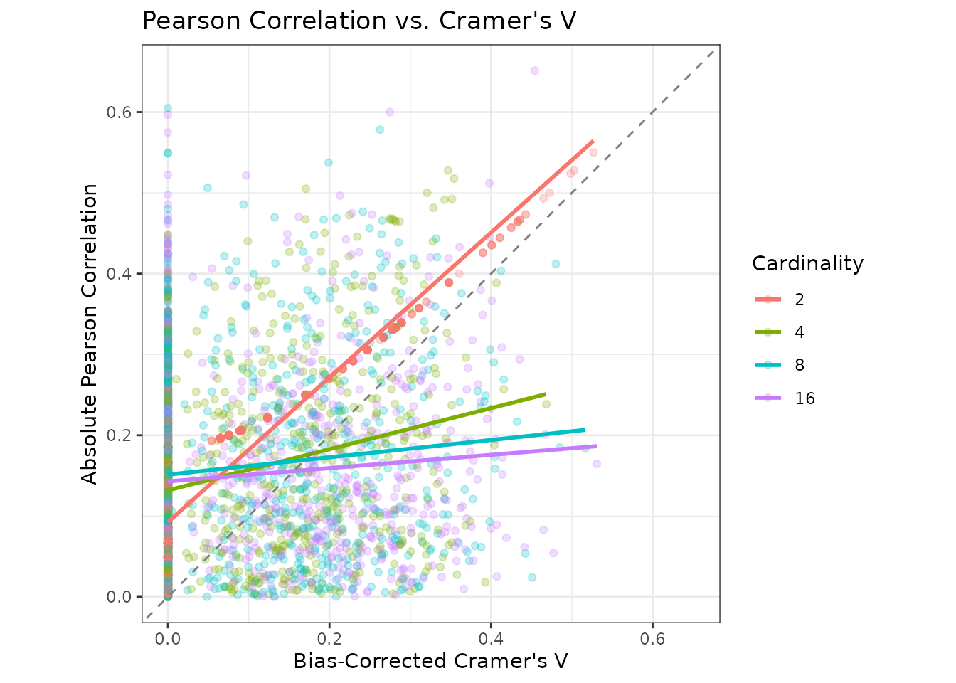
Notice how the relationship between Cramer’s V and Pearson correlation is tight for binary variables, but deteriorates rapidly as cardinality increases.

Moreover, Cramer’s V tends to produce smaller values than Pearson’s correlation. This creates a systematic bias favoring categorical predictors in multicollinearity analysis when the two measures are compared directly.

To make users aware of this issue, the function returns either a message or a warning.

The message appears when there are at least two categorical and one numeric predictor and quiet = FALSE.

x <- collinear::cor_df(
  df = vi_smol,
  predictors = predictors,
  quiet = FALSE
)
#> 
#> collinear::cor_df(): 2 categorical predictors have cardinality > 2 and may bias the multicollinearity analysis. Applying target encoding to convert them to numeric will solve this issue.

The warning appears when quiet = TRUE.

x <- collinear::cor_df(
  df = vi_smol,
  predictors = predictors,
  quiet = TRUE
)
#> Warning: 
#> collinear::cor_df(): 2 categorical predictors have cardinality > 2 and may bias the multicollinearity analysis. Applying target encoding to convert them to numeric will solve this issue.

Recommendations

Based on the analysis above, here are practical recommendations:

1. For numeric predictors only: Use cor_df() without concerns, as this represents the best-case scenario.

2. For mixed predictors with low-cardinality categoricals: cor_df() works well as-is, though be aware of slight underestimation in Cramer’s V values.

3. For high-cardinality categoricals:

   • Consider using target_encoding_lab() to convert them to numeric before analysis.
   • Alternatively, use collinear() with encoding_method = "loo", which handles this automatically.
   • This provides more reliable multicollinearity assessment.