Adaptive Filtering Thresholds
Source:vignettes/articles/adaptive_filtering_thresholds.Rmd
adaptive_filtering_thresholds.RmdSource Code
You can download the Rmarkdown notebook used to render this article
here.
To download the file, use the button Download raw file on the
upper-right hand of the Code panel.
Summary
The function collinear() automatically configures
multicollinearity filtering thresholds when the arguments
max_cor and max_vif are not specified.
This adaptive approach has several advantages:
- Eliminates the guesswork of choosing threshold values.
- Adapts filtering intensity to the correlation structure of the data.
- Keeps output VIF bounded within sensible limits (approximately 2.5 to 7.5).
- Allows manual override when specific thresholds are needed.
This approach was validated across 10,000 simulated datasets with varying correlation structures and predictor counts, consistently producing output VIF values in the 2–7 range while retaining informative predictors.
This article explains how the automatic threshold configuration works, demonstrates its effectiveness across varied datasets, and provides guidance on when manual configuration might be preferred.
Setup
This article requires the following packages, setup, and example data.
library(spatialData)
library(collinear)
library(future)
library(viridis)
library(ggplot2)
library(patchwork)
library(rstudioapi)

#parallelization setup
#only useful for categorical predictors
future::plan(
  future::multisession,
  workers = future::availableCores() - 1
)

#progress bar (does not work in Rmarkdown)
#progressr::handlers(global = TRUE)

data(
  vi_smol,
  vi_predictors,
  package = "spatialData"
  )

vi_predictors_numeric <- collinear::identify_numeric_variables(
  df = vi_smol,
  predictors = vi_predictors
)$valid

#example data
data(
  #dataframes with experiment data
  experiment_adaptive_thresholds,
  experiment_cor_vs_vif,
  #pre-trained GAM model
  gam_cor_to_vif
  )
Adaptive Threshold Selection
The arguments max_cor and max_vif define
the maximum pairwise correlation and variance inflation factors allowed
during multicollinearity filtering.
Unlike collinear_select(), cor_select(),
and vif_select(), which use fixed defaults
(max_cor = 0.7, max_vif = 5), the function
collinear() sets these to NULL and computes
appropriate thresholds from the data.
Let’s see how that works.
The vector vi_predictors_numeric
names numeric predictors with a moderate multicollinearity, as the stats
below show.
collinear::collinear_stats(
  df = vi_smol,
  predictors = vi_predictors_numeric
) |>
  dplyr::filter(
    statistic %in% c("quantile_0.75", "maximum")
  )
#>
#> collinear::collinear_stats()
#> └── collinear::validate_arg_df()
#>     └── collinear::drop_geometry_column(): dropping geometry column from 'df'.
#>        method     statistic    value
#> 1 correlation quantile_0.75   0.5646
#> 2 correlation       maximum   0.9919
#> 3         vif quantile_0.75 358.5660
#> 4         vif       maximum 564.8668
Notice that the VIF scores are very large! To fix this issue can run
these predictors through collinear().
x <- collinear::collinear(
  df = vi_smol,
  predictors = vi_predictors_numeric
)
#>
#> collinear::collinear()
#> └── collinear::validate_arg_df()
#>     └── collinear::drop_geometry_column(): dropping geometry column from 'df'.
#>
#> collinear::collinear(): setting 'max_cor' to 0.5711.
#>
#> collinear::collinear(): setting 'max_vif' to 3.9685.
#>
#> collinear::collinear()
#> └── collinear::validate_arg_preference_order()
#>     └── collinear::preference_order(): ranking 47 'predictors' from lower to higher multicollinearity.
#>
#> collinear::collinear(): selected predictors:
#>  - topo_elevation
#>  - topo_slope
#>  - soil_clay
#>  - humidity_range
#>  - cloud_cover_range
#>  - soil_silt
#>  - rainfall_min
#>  - swi_max
#>  - soil_soc
#>  - rainfall_max
#>  - solar_rad_range
#>  - solar_rad_max
The first two messages above indicate the values of
max_cor and max_vif selected by
collinear() based on the data properties (more about that
later).
The last message indicates the predictors selected in this run. Their stats are shown below.
collinear::collinear_stats(
  df = x$result$df,
  predictors = x$result$selection
) |>
  dplyr::filter(
    statistic %in% c("quantile_0.75", "maximum")
  )
#>        method     statistic  value
#> 1 correlation quantile_0.75 0.2929
#> 2 correlation       maximum 0.5631
#> 3         vif quantile_0.75 2.3006
#> 4         vif       maximum 3.2638
These stats show much more reasonable VIF scores now.
However, if you are aiming for specific multicollinearity thresholds,
the automatic setup can be overriden by providing the desired values for
max_cor and/or max_vif. If one of them is not
defined, it will be ignored.
x <- collinear::collinear(
  df = vi_smol,
  predictors = vi_predictors_numeric,
  max_cor = 0.5,
  max_vif = 2.5
)
#>
#> collinear::collinear()
#> └── collinear::validate_arg_df()
#>     └── collinear::drop_geometry_column(): dropping geometry column from 'df'.
#>
#> collinear::collinear()
#> └── collinear::validate_arg_preference_order()
#>     └── collinear::preference_order(): ranking 47 'predictors' from lower to higher multicollinearity.
#>
#> collinear::collinear(): selected predictors:
#>  - topo_elevation
#>  - topo_slope
#>  - soil_clay
#>  - humidity_range
#>  - cloud_cover_range
#>  - soil_silt
#>  - rainfall_min
#>  - swi_max
#>  - soil_nitrogen
#>  - solar_rad_range

collinear::collinear_stats(
  df = x$result$df,
  predictors = x$result$selection
) |>
  dplyr::filter(
    statistic %in% c("quantile_0.75", "maximum")
  )
#>        method     statistic  value
#> 1 correlation quantile_0.75 0.2711
#> 2 correlation       maximum 0.4754
#> 3         vif quantile_0.75 1.6726
#> 4         vif       maximum 1.7726
By adapting thresholds to each dataset’s structure,
collinear() provides sensible defaults while still allowing
manual override when needed.
Validation
To validate this adaptive threshold selection method I ran
collinear() on 10,000 random subsets of a synthetic dataset
with 500 columns and 10,000 rows generated using
distantia::zoo_simulate(). Each iteration randomly selected
10-100 predictors and 30-100 rows per predictor, then compared input and
output multicollinearity statistics.
The experiment script can be opened in RStudio as follows:
system.file(
  "experiments/validation_adaptive_thresholds.R",
  package = "collinear"
  ) |>
  rstudioapi::navigateToFile()
The results of this experiment are in the dataframe experiment_adaptive_thresholds,
plotted below.
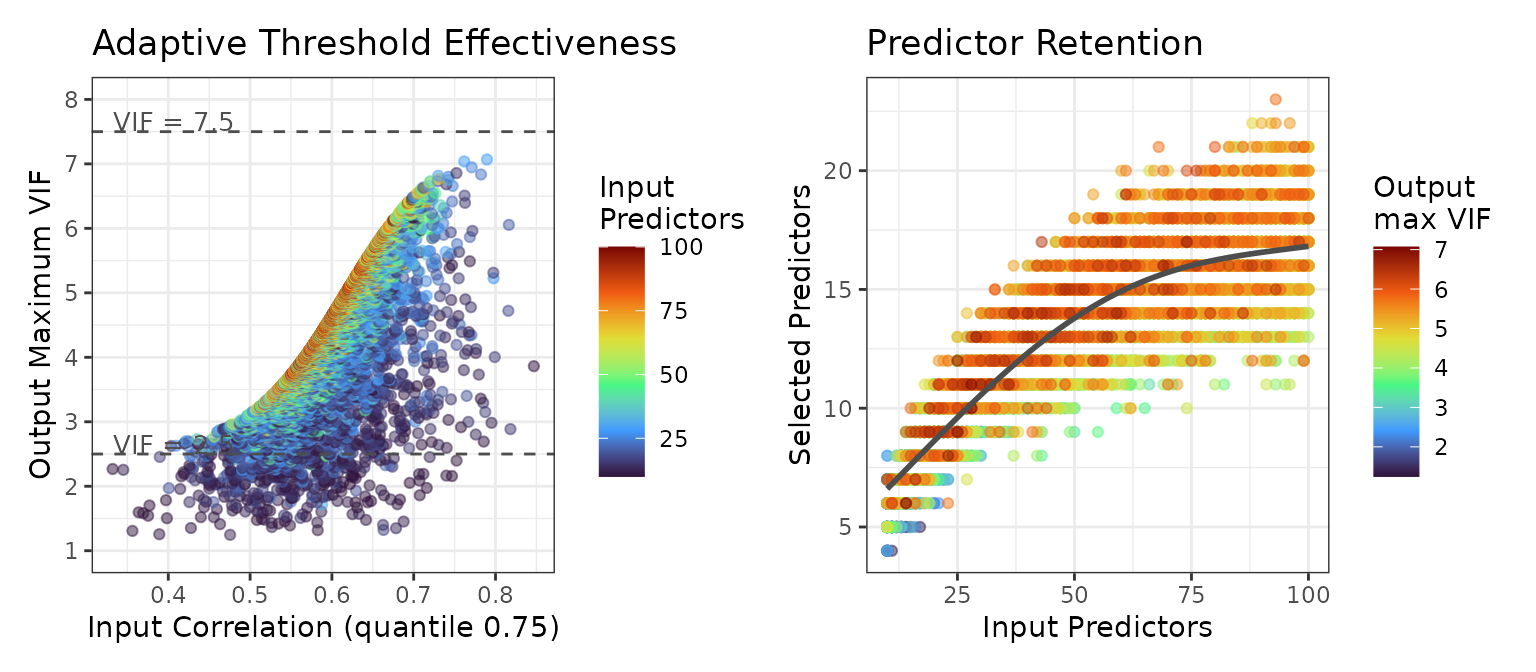
The left panel shows the 75th percentile of input correlation against the maximum VIF of the resulting selection. The cases below the VIF = 2.5 line (4% of all cases) are datasets with a small number of predictors where multicollinearity drops sharply when one or several key predictors are removed
The right panel shows the number of predictors before and after multicollinearity filtering. The sublinear relationship indicates that even with 100 input predictors, the selection stabilizes around 15-20 predictors.
These results indicate that the adaptive threshold selection works well across most use cases.
Step By Step
The adaptive selection of multicollinearity thresholds requires three steps:
1. Compute the quantile 0.75 of the correlation for
the input predictors via cor_stats(). This quantile is used
because it captures the upper tail of the correlation distribution,
where the problematic multicollinearity begins.
cor_0.75 <- collinear::cor_stats(
  df = vi_smol,
  predictors = vi_predictors_numeric,
  quiet = TRUE
) |>
  dplyr::filter(statistic == "quantile_0.75") |>
  dplyr::pull(value)

cor_0.75
#> [1] 0.5646
2. Sigmoid transformation of the
cor_0.75 value. This sigmoid function smoothly maps the
input correlation to a bounded max_cor threshold.
max_cor <- 0.493 + 0.242 / (1 + exp(-15 * (cor_0.75 - 0.614)))

max_cor
#> [1] 0.5711141
Where:
-
0.493: floor of the curve, corresponding to VIF ≈ 2.5 inprediction_cor_to_vif(conservative filtering). -
0.735: ceiling of the curve (0.545 + 0.24), corresponding to VIF ≈ 7.5 inprediction_cor_to_vif(permissive filtering). -
0.614: midpoint where the transition is steepest. -
-15: steepness parameter controlling how sharply the curve transitions.
The full sigmoid curve is shown below.
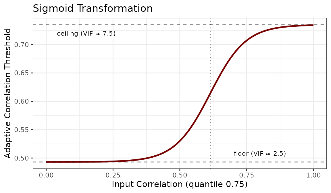
Datasets with low correlation (quantile 0.75 < 0.5) receive thresholds near the floor, while highly correlated datasets (quantile 0.75 > 0.8) approach the ceiling. This prevents both over-filtering of clean datasets and under-filtering of problematic ones.
- The pre-trained GAM model
gam_cor_to_vifpredicts a suitablemax_viffrom themax_corresulting from the transformation.
max_vif <- mgcv::predict.gam(
  object = collinear::gam_cor_to_vif,
  newdata = data.frame(max_cor = max_cor)
)

max_vif
#>        1
#> 3.968778
This model was fitted on the simulation results in experiment_cor_vs_vif,
where both filtering methods were applied across 10,000 random dataset
configurations. For each max_cor value, the
max_vif producing the highest Jaccard similarity between
the two selections was identified.
The experiment script can be opened in RStudio as follows:
system.file(
  "experiments/relationship_cor_vs_vif.R",
  package = "collinear"
) |>
  rstudioapi::navigateToFile()
The model uses squared Jaccard similarity as weights to emphasize
cases where cor_select() and vif_select()
achieved strong agreement.
m <- mgcv::gam(
  formula = max_vif ~ s(max_cor, k = 6),
  weights = experiment_cor_vs_vif$out_selection_jaccard^2,
  data = experiment_cor_vs_vif
)
The plot below shows the simulation results and the fitted model.
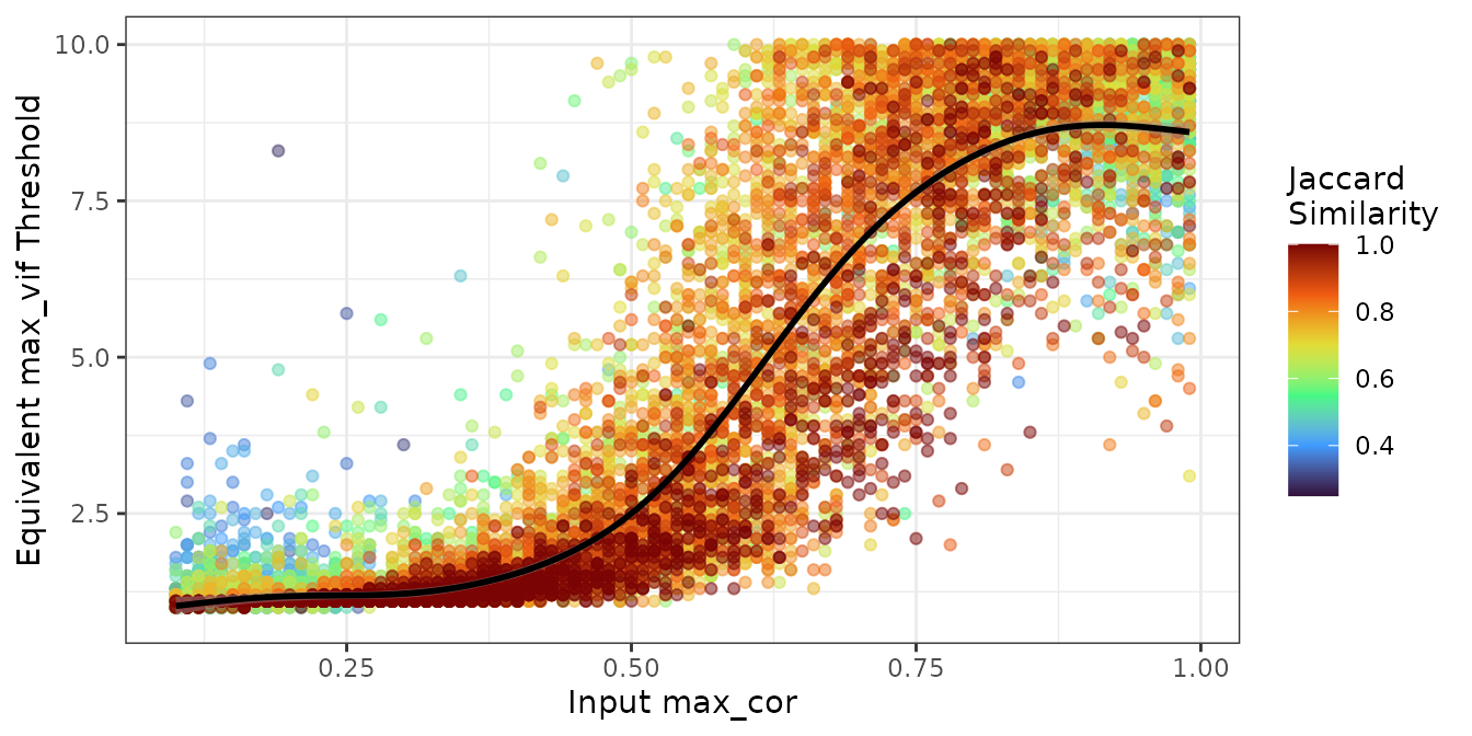
The curve tracks through the high-similarity region (red/orange
points), indicating that the model successfully captures the
relationship between max_cor and max_vif for
cases where both methods agree.
When to Override
While the adaptive defaults work well for most cases, consider setting thresholds manually when:
Strict coefficient interpretability is required: Set
max_vif = 2.5or lower for models where coefficient stability is critical.Maximizing predictor retention: Set
max_cor = 0.9andmax_vif = 10for prediction-focused models where some multicollinearity is acceptable.Domain-specific requirements: Some fields have established VIF thresholds (e.g., VIF < 5 or VIF < 10) that should be used for consistency with existing literature.