Summary

This document describes in detail how to analyze ecological memory patterns present in simulated pollen curves generated with the virtualPollen and memoria packages. First, we describe the complex statistical properties of the virtual pollen curves produced by virtualPollen and how these may impact ecological memory analyses; Second we explain how Random Forest works, from its basic components (regression trees) to the way in which it computes variable importance; Third, we explain how to analyze ecological memory patterns on the simulation outputs.

The model

Analyzing ecological memory requires to fit a model of the form:

Equation 1 (simplified from the one in the paper): \[p_{t} = p_{t-1} +...+ p_{t-n} + d_{t} + d_{t-1} +...+ d_{t-n}\]

Where:

\(p\) is Pollen.
\(d\) is Driver.
\(t\) is the time of any given value of the response \(p\).
\(t-1\) is the lag 1.
\(p_{t-1} +...+ p_{t-n}\) represents the endogenous component of ecological memory.
\(d_{t-1} +...+ d_{t-n}\) represents the exogenous component of ecological memory.
\(d_{t}\) represents the concurrent effect of the driver over the response.

The function prepareLaggedData shown below organizes the input data in lags. It requires to identify what columns in the original data should act as response, drivers, and time, and what lags are to be generated.

#loading data
data(simulation) #from virtualPollen
sim <- simulation[[1]]

#generating vector of lags (same as in paper)
lags <- seq(20, 240, by = 20)

#organizing data in lags
sim.lags <- prepareLaggedData(
  input.data = sim,
  response = "Pollen",
  drivers = c("Driver.A", "Suitability"),
  time = "Time",
  lags = lags,
  scale = FALSE
  )

This function returns the data shown in Table 1. This kind of data structure is known as lagged data or time delayed data. Note that the function can use a scale argument (set to FALSE above) to standardize the data before generating the lags. Random Forest does not generally require standardization to fit accurate models of the data, but computing variable importance with variables having large differences in range (i.e. [1, 10] vs. [1, 10000]) might yield biased results, making standardization a recommended step in data preparation. In this appendix all data are shown without any standardization to let the reader to keep track of the different variables across analyses and have a sense of their magnitude, but note that all analyses presented in the paper were based on standardized data.

The data in Table 1 are organized to fit the model described by Equation 1, but to select a proper method to fit the model, three main features of the data have to be considered first: temporal autocorrelation, multicollinearity, and non-linearity.

The data

The simulations produced by virtualPollen have some key properties that justify the use of Random Forest as analytical tool.

Temporal autocorrelation

Temporal autocorrelation (also serial correlation) refers to the relationship between successive values of the same variable present in most time series. Temporal autocorrelation generates autocorrelated residuals in regression analysis, violating the assumption of “independence of errors” required to correctly interpret regression coefficients. Several methods can be used to address temporal autocorrelation in regression analysis, such as increasing time intervals between consecutive samples, or incorporating an auto-regressive structure into the model.

Every variable used in our study presents this characteristic. The driver was generated with a temporal autocorrelation significant for periods of 600 years. The suitability produced by the niche function of the virtual taxa based on the values of the driver also presents temporal autocorrelation, but generally lower than the one of the driver. Finally, the response, since it is the result of a dynamic model in which every data-point depends on the previous one, also shows a temporal structure, which varies depending on the taxa’s traits, as so does the suitability (see Figure 2).

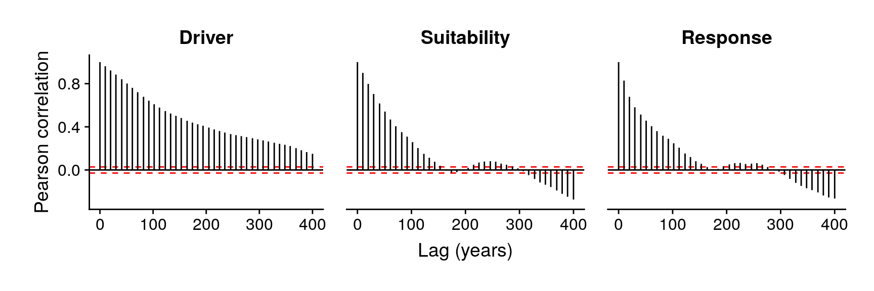
Temporal autocorrelation of the variables in the example data.

Multicollinearity

Multicollinearity occurs when there is a high correlation between predictors in a model definition. It increases the standard error of the coefficients, meaning that their estimates for important predictors can become statistically insignificant, wildly impacting model interpretation.

Adding consecutive time-lags of the same variables to the data, as required by the model expressed in Equation 1 largely increases multicollinearity.

Non-linearity

The function virtualPollen::simulatePopulation has the ability to produce pollen abundances variably decoupled from environmental conditions depending on the life-traits and niche features of the virtual taxa considered. This model property increases the chance of finding non-linear relationships between time-lagged predictors and the response (see Figure 3), hindering the detection of meaningful relationships with methods not able to account for non-nonlinearity.

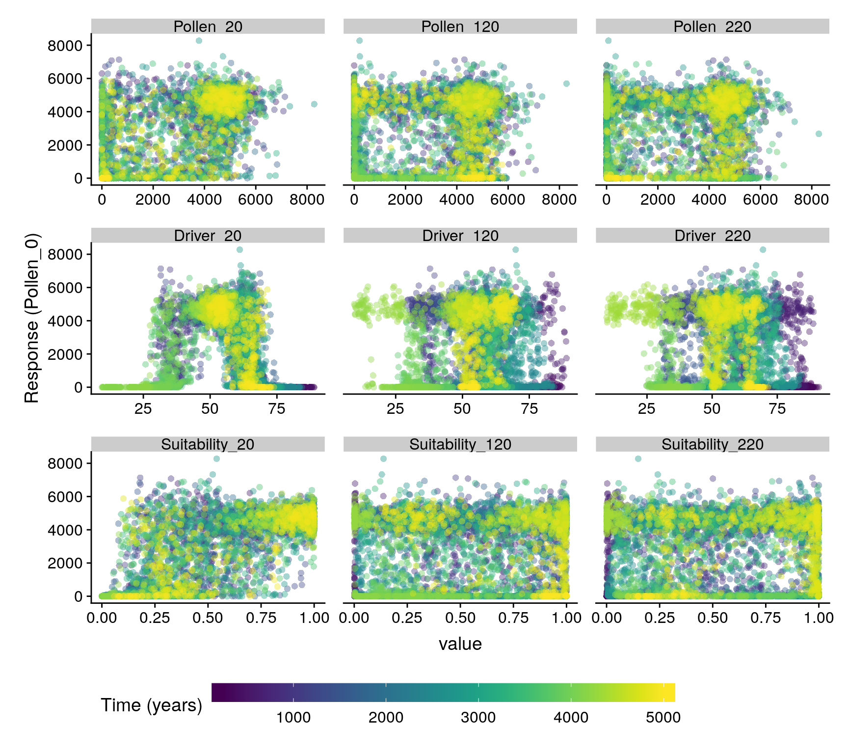
Linear and non-linear relationships arising from lagged data in the annual dataset.

The logics behind Random Forest

The trees

The fundamental units of a Random Forest model are regression trees. A regression tree grows through binary recursive partition. Considering a response variable, and a set of predictive variables (also named features in the machine learning language), the following steps grow a regression tree:

For each variable, the point in their ranges that optimizes the separation (partition) of the response in two groups of cases is searched for. The selected point minimizes the sum of the squared deviations from the mean in the two separated partitions.
The variable with the lower sum of the squared deviations from the means is selected as the root node of the tree, and the data are separated in two partitions, one on each side of the split value of the given variable.
The steps above are recursively applied to each partition to create new partitions, until all cases are in partitions that can be no longer separated in smaller partitions because they are too homogeneous, or because they have reached a minimum sample size. These final partitions are named terminal nodes.

The code below shows how to fit a recursive partition tree with the rpart library on the first lag (20 years) of pollen and driver of the data shown in Figure 2.

#fitting model (only two predictors)
rpart.model <- rpart(
  formula = Response_0 ~ Response_20 + Driver.A_20,
  data = sim.lags,
  control = rpart.control(minbucket = 5)
  )

#plotting tree
rpart.plot(
  rpart.model, 
  type = 0, 
  box.palette = viridis(10, alpha = 0.2)
  )

Recursive partition tree (also regression tree) of pollen abundance (noted as Response_0 in the model) as a function of Response_20 (antecedent pollen abundance at lag 20) and Driver_20 (antecedent driver values at lag 20). Numbers in branches represent split values, while numbers in terminal nodes represent the predicted average for that particular node. Percentages represent the relative number of cases included in each terminal node.

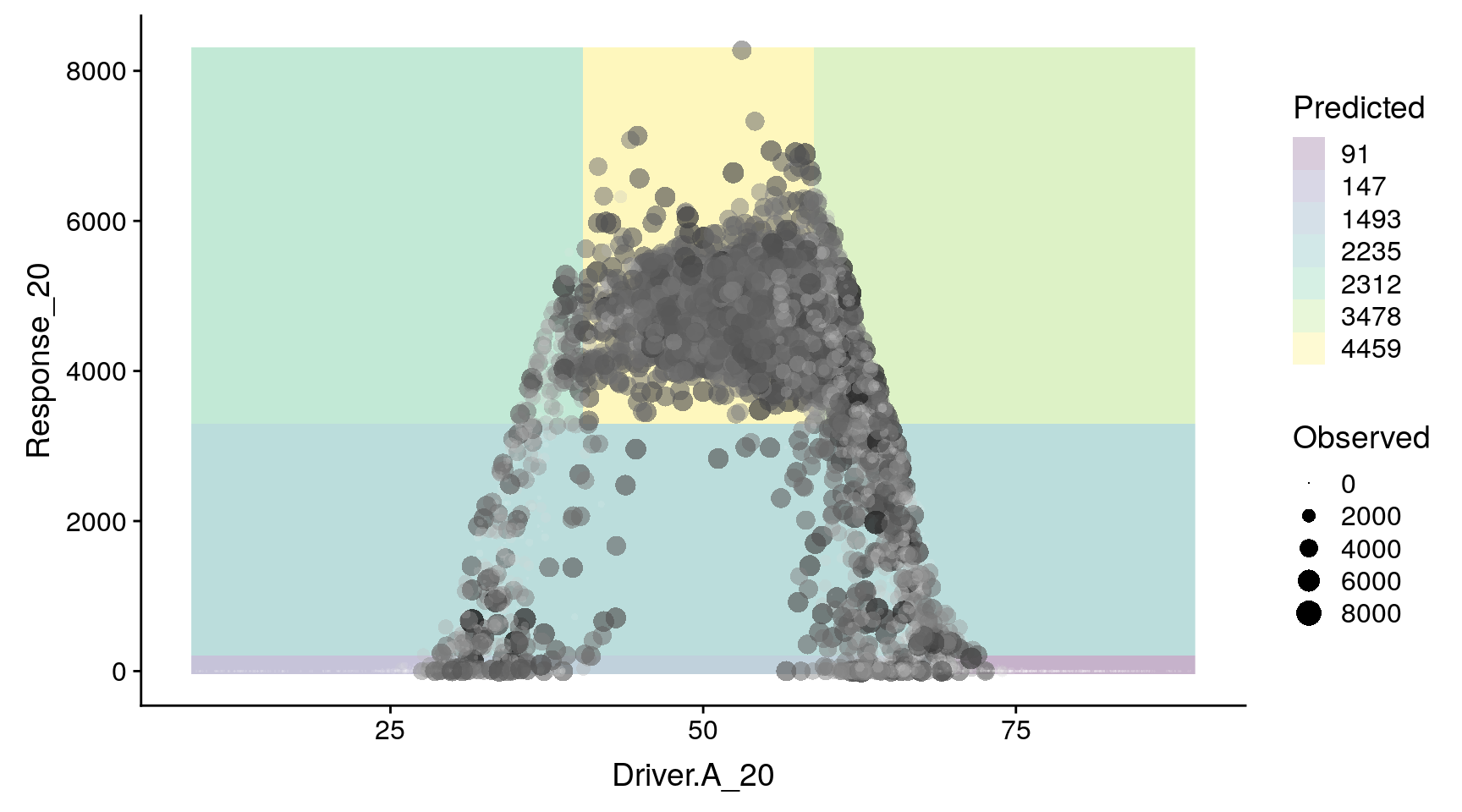
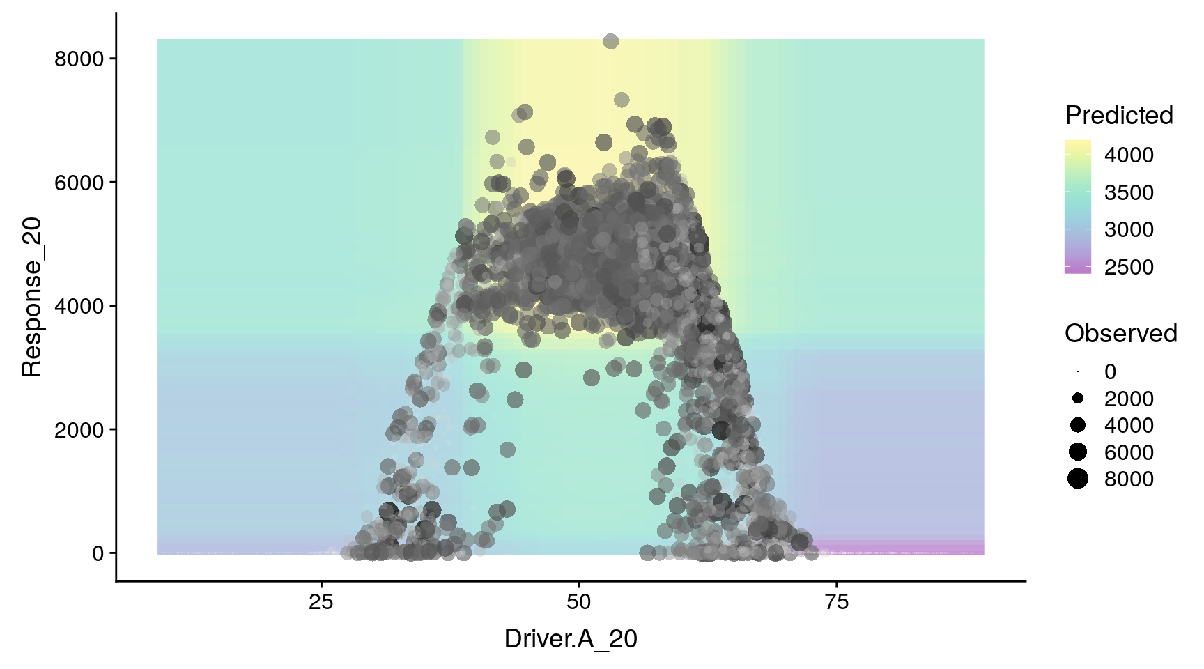
Recursive partition surface generated by the model fitted above. Dots represent observed data, and colours identify partitions shown in the recursive partition tree. Note that this partition surface can be generalized to any number of predictors/dimensions.

Figure 4 shows the recursive partition tree fitted on Pollen_0 as a function of the first lag of pollen (Pollen_20) and the driver (Driver_20), while Figure 5 shows the partitions in the space of both variables. As shown in both figures, the recursive partition tree is, in essence, separating the cases into regions in which given combinations of the predictors lead to certain average values of the response. The tree also shows the hierarchy in importance between both predictors, with Pollen_20 defining all splits but one. Only when Pollen_20 is higher than 3772, the variable Driver_20 becomes important, indicating that maximum abundances are only reached after that point, and only if Driver_20 has a value lower than 71. This is how partial interactions among predictors are expressed in recursive partition trees.

The tree has grown until data in the terminal nodes cannot be separated further into additional partitions, or has reached the minimum number of cases defined by the variable minbucket. The minimum amount of cases in a terminal node defines the overall resolution of the model. Smaller numbers lead to a higher amount of terminal nodes, and therefore to more partitions in the data space. This can be confirmed by changing the minbucket value in the code above, and assessing subsequent changes in tree structure and number of partitions.

As a drawback, the splits of a recursive partition trees are highly sensitive to small changes in the input data, specially when sample size is small. This instability has led to the development of more sophisticated methods to fit recursive partition trees, such as conditional inference trees (see function ctree in library partykit), or ensemble methods such as Random Forest.

The forest

A Random Forest model is composed by a large number of individual regression trees (500 or more) generated on random subsamples of the predictors and the cases. For a random set of cases, each tree is fitted as follows:

A random subset of predictors of size mtry is selected. The default mtry is the rounded-up squared root of the total number of predictors, but the user can modify it.
The predictor from the random subset that better separates the data into two partitions is selected as root node, an the data are separated in two partitions, one at each side of the split value.
On each partition, a new random subset of predictors of size mtry is selected (and this is the main difference between a recursive partition tree and a Random Forest tree, the former uses all variables on each split), and again the predictor that better separates the partition into two new partitions is selected, and new partitions are defined.
The tree is grown until minimum node size is reached in all terminal nodes, or no further partitions can be defined.
The tree is evaluated by computing its mean squared error (mse) on the ~37% of the data not used to train it (named out-of-bag data).
For each variable in the tree the algorithm performs a permutation test as follows:
- The column with the given variable is randomly permuted.
- A new tree is fitted with the permuted variable.
- Mean squared error is computed again on the out-of-bag data.
- Difference in mse between the tree fitted with the original variable and the tree fitted with the permuted one is computed and stored.

Once all trees have been fitted, for every given case, the prediction is computed as the mode of the individual predictions of every tree (but not the ones fitted with permuted variables). The importance of every variable is computed as the average of the differences in mean squared error between trees computed with the variable and trees computed with the permuted variable, normalized by the standard deviation of the differences.

Random Forest does not require any assumptions to be fulfilled by the data or the model outcomes, and therefore it can be applied to a wide range of analytic cases where data are non-linear. As a drawback, the randomness in the selection of cases and predictors to fit individual regression trees turns it into a non-deterministic algorithm, and therefore, fine-scale variations in the outcomes are to be expected between different runs with the same data.

To fit Random Forest models on the simulated data we selected the package ranger over the more traditional randomForest because the former allows multithread computing (uses all available cores in a computer while fitting the forest), achieving a better performance for large datasets than the later. The code below shows how to use ranger to fit a Random Forest model.

#getting columns containing "Response" or "Driver"
sim.lags.rf <- sim.lags[, grepl("Driver|Response", colnames(sim.lags))]

#fitting a Random Forest model
rf.model <- ranger(
  data = sim.lags.rf,
  dependent.variable.name = "Response_0",
  num.trees = 500,
  min.node.size = 5, 
  mtry = 2,
  importance = "permutation", 
  scale.permutation.importance = TRUE)

#model summary
print(rf.model)

#R-squared (computed on out-of-bag data)
rf.model$r.squared

#variable importance
rf.model$variable.importance

#obtain case predictions
rf.model$predictions

#getting information of the first tree
treeInfo(rf.model, tree=1)

The function ranger has the following key arguments:

data: dataframe with the variables to be included in the model.
dependent.variable.name: model definition can be done in two ways, either through a formula, or through the argument dependent.variable.name, that names the response variable, and uses the remaining variables in the dataset as predictors, which forces us to be careful with what variables are available in the dataset.
num.trees: controls number of trees generated (the default value is 500).
mtry: controls the number of variables randomly selected to fit each tree. In the code above this argument is set to 2, indicating that the model only considers interactions among two predictors only on each tree. This allows to compute variable importance as independently as possible from other variables.
min.node.size: minimum number of cases in a terminal node, which determines the overall resolution of the model.
importance: when set to “permutation” it triggers the computation of variable importance through permutation tests.
scale.permutation.importance: scales importance values computed through the permutation tests by the overall standard error.

The relationship between the response variable and the predictors can be examined through partial dependence plots (see Figure 6). A partial dependence plot is a simplified view of the inner structure of the model. Since regression trees consider interactions among variables, the prediction for any given case depends on the values of all predictors considered at the same time. Since it is not possible to generate such a representation in 2D or 3D, partial dependence plots set all variables not represented in the plot to their respective means. Therefore, partial dependence plots must be interpreted as simple approximations to the true shape of the model surface.

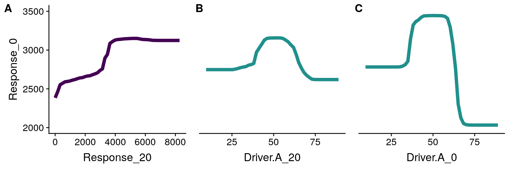
Partial dependence plots of the lags 20, of Pollen (A) and Driver (B), and the concurrent effect (Driver_0, panel C).

Interactions among predictors can be represented in the same way done before for recursive partition trees (see Figure 7). Again, all variables not represented in the plot are set to their average to generate the prediction.

Interaction between Pollen_20 (first lag of the endogenous memory) and Suitability_0 (concurrent effect).

Variable importance

Random forest variable importance computation works under the assumption that if a given variable is not important, then permuting its values does not degrade the prediction accuracy. Variable importance scores are extracted with the importance function (see code below and Table 4), and are interpreted as “how much model fit degrades when the given variable is removed from the model”.

importance(rf.model)

Values shown in Table 4 are the result of one particular Random Forest run. For variables with small differences in importance, the ranking shown in the table could change in a different model run. This situation can be addressed by running the model several times, and computing the average and confidence intervals of the importance scores of each predictor across runs. This is shown in the code below (see output in Figure 8).

#number of repetitions
repetitions <- 10

#list to save importance results
importance.list <- list()

#repetitions
for(i in 1:repetitions){
  
  #fitting a Random Forest model
  rf.model <- ranger(
    data = sim.lags.rf,
    dependent.variable.name = "Response_0",
    mtry = 2,
    importance = "permutation", 
    scale.permutation.importance = TRUE
    )

  #extracting importance
  importance.list[[i]] <- data.frame(t(importance(rf.model)))
}

#into a single dataframe
importance.df <- do.call("rbind", importance.list)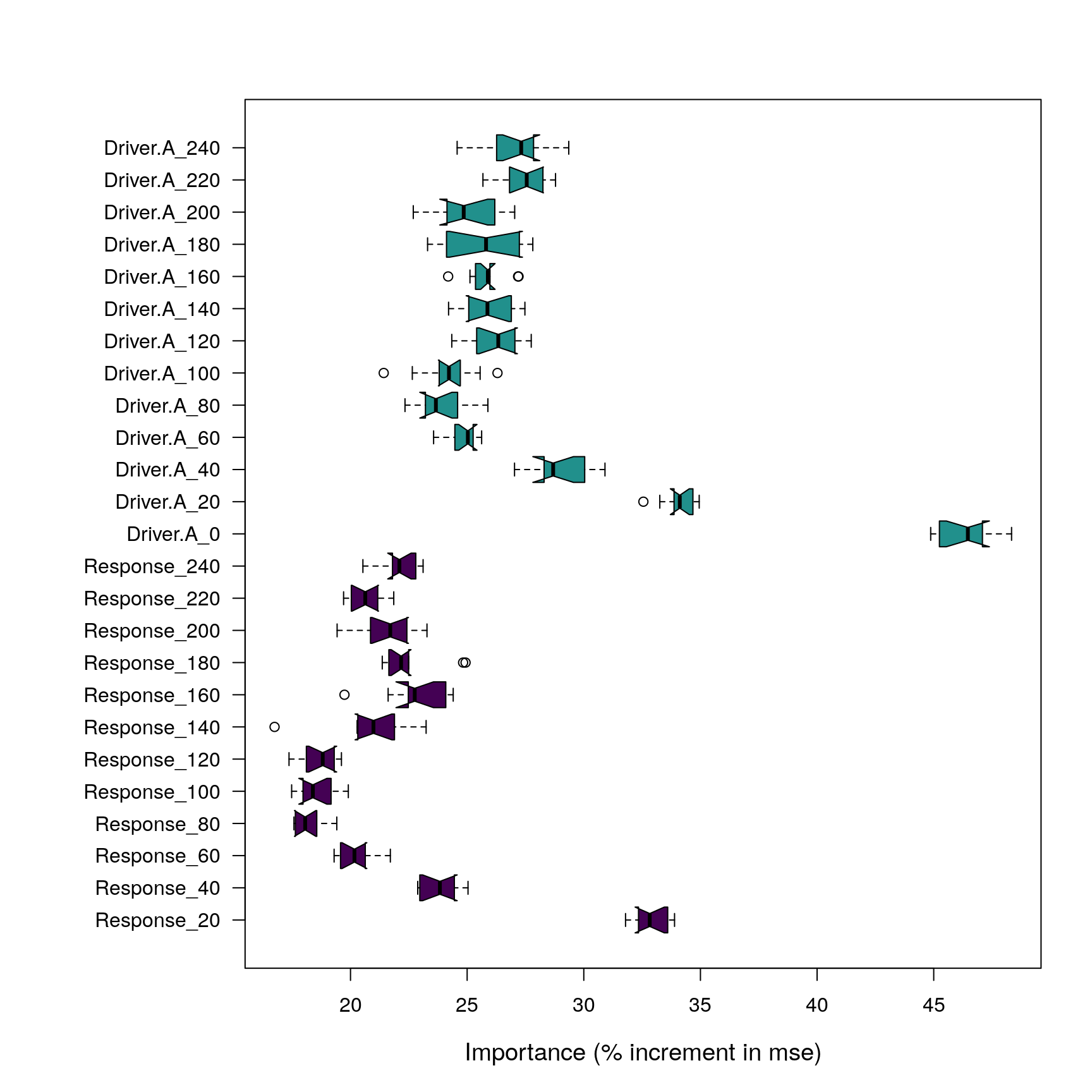

Importance scores of predictors in Random Forest model after 100 repetitions. Note that Response_X predictor refers to the endogenous memory, and Driver_X predictors from lag 20 refer to exogenous memory. Driver_0 represents the concurrent effect.

Testing the significance of variable importance scores

Random Forest does not provide any tool to assess the significance of these importance scores, and it is therefore impossible to know at what point they become irrelevant. A simple solution is to add a random variable as an additional predictor to the model and compute its importance. If the importance of other variables is equal or lower than the importance of the random variable, it can be assumed that these variables do not have a meaningful effect on the response, and can therefore be considered irrelevant.

Two types of random variables can be considered to be used as benchmarks to test variable importance scores provided by Random Forest: white noise (without any temporal structure), and random walk with temporal structure (as explained in Appendix I). In both cases the idea is to generate a null model providing a baseline to assess to what extent importance scores are higher than what is expected by chance. To test the suitability of both methods, the code below generates 10 Random Forest models, each one with two additional random variables: random.white representing white noise, and random.autocor representing an autocorrelated random walk. The length of the autocorrelation period of random.autocor is changed for every iteration.

#number of repetitions
repetitions <- 10

#list to save importance results
importance.list <- list()

#rows of the input dataset
n.rows <- nrow(sim.lags.rf)

#repetitions
for(i in 1:repetitions){
  
  #adding/replacing random.white column
  sim.lags.rf$random.white <- rnorm(n.rows)
  
  #adding/replacing random.autocor column
  #different filter length on each run = different temporal structure
  sim.lags.rf$random.autocor <- as.vector(
    filter(rnorm(n.rows),
           filter = rep(1, sample(1:floor(n.rows/4), 1)),
           method = "convolution",
           circular = TRUE))

  #fitting a Random Forest model
  rf.model <- ranger(
    data = sim.lags.rf,
    dependent.variable.name = "Response_0",
    mtry = 2,
    importance = "permutation", 
    scale.permutation.importance = TRUE)

  #extracting importance
  importance.list[[i]] <- data.frame(t(importance(rf.model)))
  
}

#into a single dataframe
importance.df <- do.call("rbind", importance.list)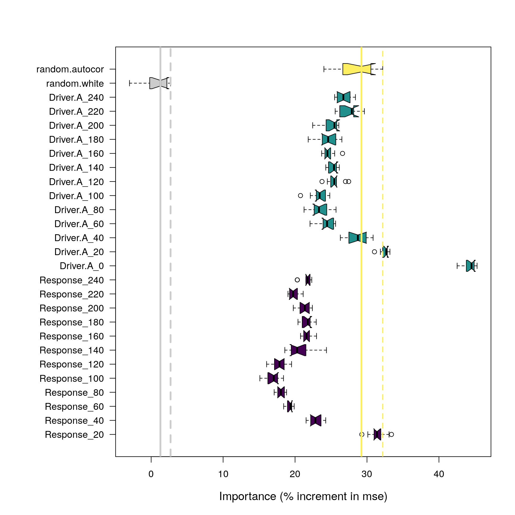

Importance of predictors in relation to the importance of a white noise variable (gray), and a temporally structured random variable (yellow). Solid lines represent the medians of the random variables, while dashed lines represent their maximum importance across 100 model runs.

The boxplot in Figure 9 shows the relative importance of the random variables, and suggests that the variable representing random noise is not useful to identify importance scores arising by chance. On the other hand, the variable based on autocorrelated random walks (marked in yellow in the plot) tells a different story. Importance values below the yellow solid line have a probability higher than 0.5 of being the result of chance. Importance values between the yellow solid and dashed lines have probabilities between 0.5 and 0 and are the result of a random association between a predictor and the response, while beyond the dashed line the results can be confidently defined as non-random. Note that Figure 8, when compared with Figure 7, also shows that adding random variables to a Random Forest model does not change the importance scores of other variables in the model.

Analyzing ecological memory with Random Forest and the memoria library

So far we have explained how to organize the simulated pollen curves in lags, and how to fit Random Forest models on the lagged data to evaluate variable importance. However, further steps are required to quantify ecological memory patterns:

Extract and aggregate variable importance scores, and organize them in ecological memory components (endogenous, exogenous, and concurrent).
Plot the pattern to facilitate interpretation.
Extract ecological memory features from these components, namely memory strength (maximum difference in relative importance between each component (endogenous, exogenous, and concurrent) and the median of the random component), memory length (proportion of lags over which the importance of a memory component is above the median of the random component), and dominance (proportion of the lags above the median of the random term over which a memory component has a higher importance than the other component).

The function computeMemory fits as many Random Forest models as indicated by the argument repetitions on a lagged dataset, and on each iteration includes a random variable in the model. The function plotMemory gets the output of computeMemory and plots it, while the function extractMemoryFeatures computes the features of each ecological memory component. The simplified workflow is shown below.

#computes ecological memory pattern
memory.pattern <- computeMemory(
  lagged.data = sim.lags, 
  drivers = "Driver.A", 
  random.mode="autocorrelated",
  repetitions=30, 
  response="Response"
  )

#computing memory features
memory.features <- extractMemoryFeatures(
  memory.pattern=memory.pattern,
  exogenous.component="Driver.A",
  endogenous.component="Response"
  )

#plotting the ecological memory pattern
plotMemory(memory.pattern)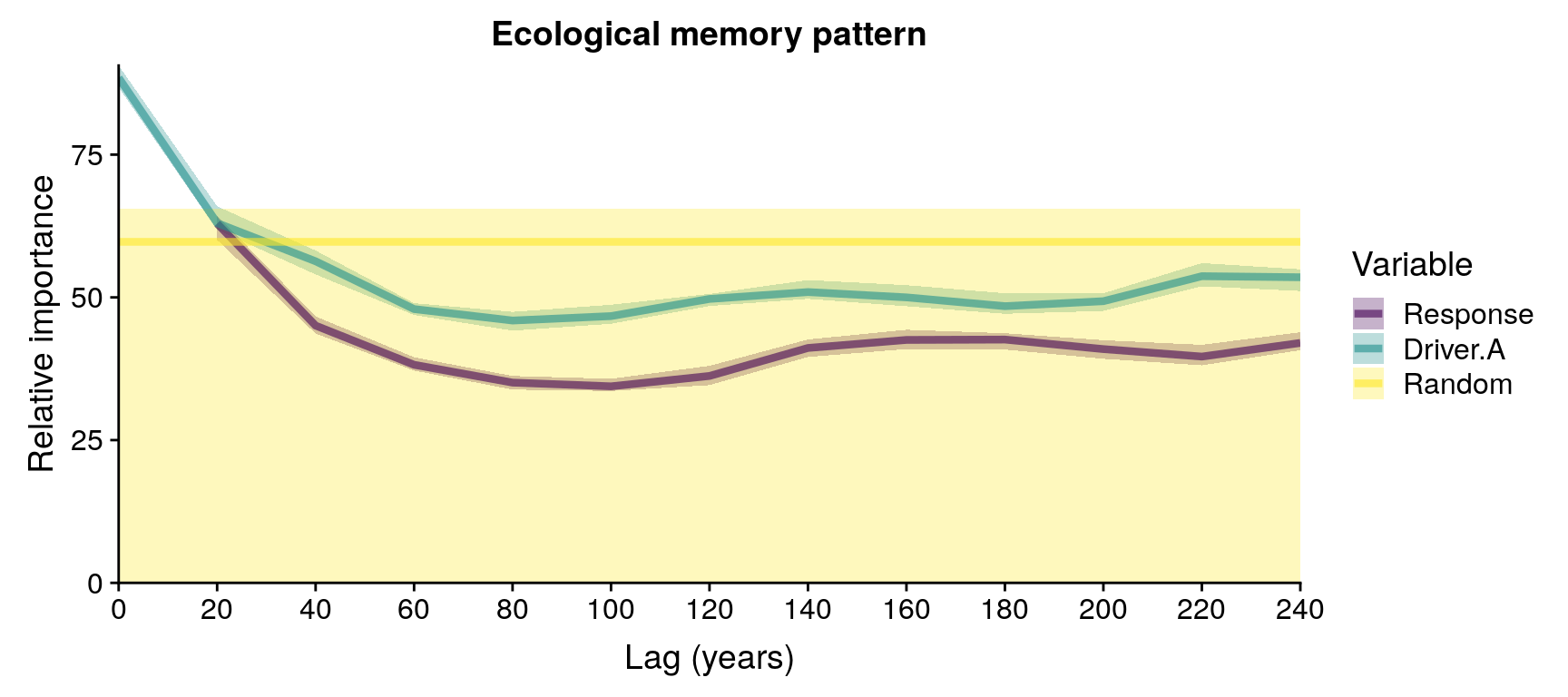

Example of ecological memory pattern. Note that the model was only run for 30 repetitions, and therefore the position of the median of the Random component is not reliable.

In order to analyze the ecological memory patterns of 16 virtual taxa across the 5 levels of data quality (Annual, 1cm, 2cm, 6cm, and 10cm), we integrated the functions above into a larger function named runExperiment. The code below runs an artificial simple example with only two virtual taxa (1 and 6 in parameters), and two dataset types (“1cm” and “10cm”). Only 30 repetitions are generated to quicken execution, which is not nearly enough to achieve consistent results.

#running experiment
E1 <- runExperiment(
  simulations.file = simulation,
  selected.rows = 1:4,
  selected.columns = 1,
  parameters.file = parameters,
  parameters.names = c("maximum.age",
                       "fecundity",
                       "niche.A.mean",
                       "niche.A.sd"),
  sampling.names = "1cm",
  driver.column = "Driver.A",
  response.column = "Pollen",
  time.column = "Time",
  lags = lags,
  repetitions = 30
  )

#E1 is a list of lists
#first list: names of experiment output
E1$names 

#second list, first element
i <- 1 #change to see other elements
#ecological memory pattern
E1$output[[i]]$memory

#pseudo R-squared across repetitions
E1$output[[i]]$R2

#predicted pollen across repetitions
E1$output[[i]]$prediction

#variance inflation factor of input data
E1$output[[i]]$multicollinearity

Experiment results can be plotted with the function plotExperiment shown below.

plotExperiment(
  experiment.output=E1,
  parameters.file=parameters,
  experiment.title="Toy experiment",
  sampling.names=c("1cm", "10cm"),
  legend.position="bottom",
  R2=TRUE
  )

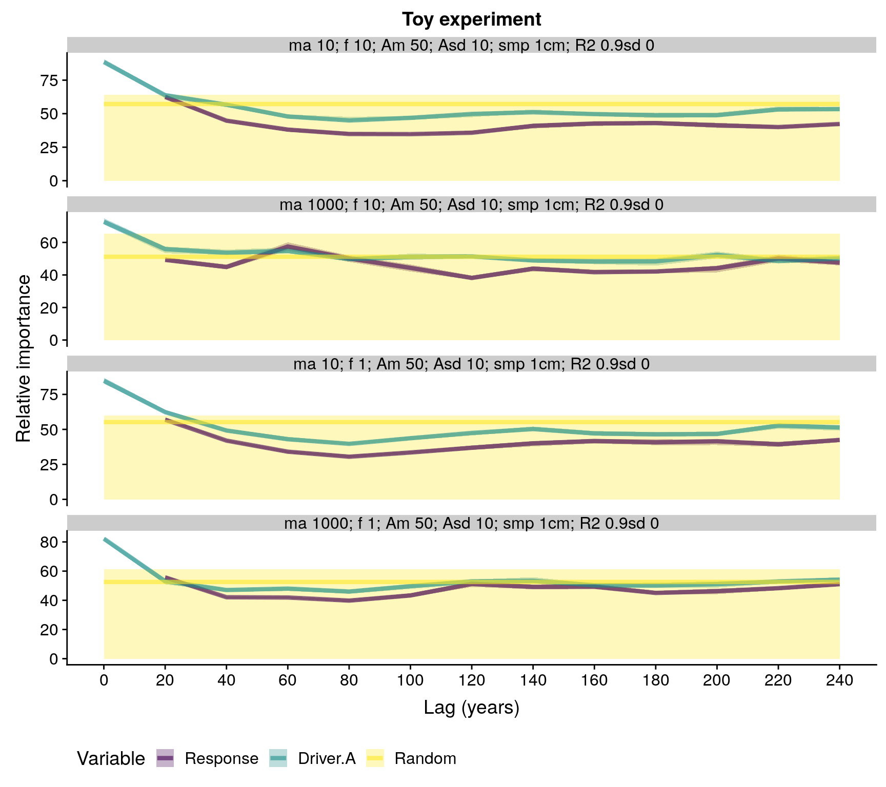
Ecological memory patterns of four virtual taxa. Note that the number of repetitions (30) is too low to obtain a reliable median of the Random component. Abbreviations in plot title: ma - maximum age, f - fecundity, Am - niche mean, Asd - niche breadth, smp - sampling resolution, R2 - pseudo R-squared.

The experiment data can be organizes as a single table, joined with the data available in the parameters dataframe to facilitate further analyses.

E1.df <- experimentToTable(
  experiment.output=E1,
  parameters.file=parameters,
  sampling.names=c("1cm", "10cm"),
  R2=TRUE
  )

Finally, ecological memory features can be extracted from the experiment with extractMemoryFeatures in order to facilitate further analyses, as shown below.

E1.features <- extractMemoryFeatures(
  memory.pattern = E1.df,
  exogenous.component = "Driver.A",
  endogenous.component = "Response"
  )

Using “memoria” and “virtualPollen” together

Quantifying ecological memory of virtual pollen curves

Blas M. Benito