Plot residuals diagnostics

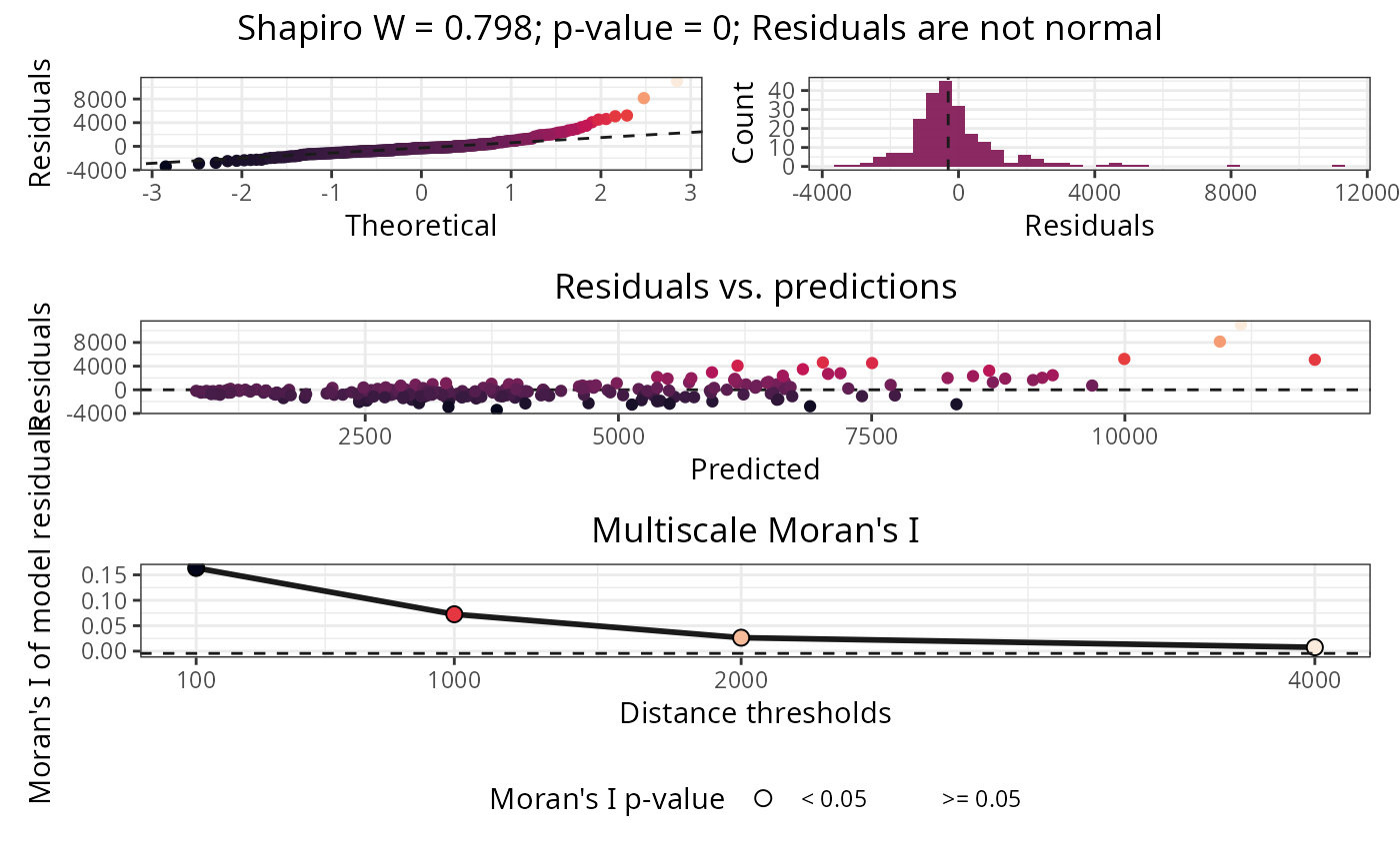
Plots normality and autocorrelation tests of model residuals.

plot_residuals_diagnostics(
  model,
  point.color = viridis::viridis(100, option = "F"),
  line.color = "gray10",
  fill.color = viridis::viridis(4, option = "F", alpha = 0.95)[2],
  option = 1,
  ncol = 1,
  verbose = TRUE
)

Arguments

model

A model produced by rf(), rf_repeat(), or rf_spatial().

point.color

Colors of the plotted points. Can be a single color name (e.g. "red4"), a character vector with hexadecimal codes (e.g. "#440154FF" "#21908CFF" "#FDE725FF"), or function generating a palette (e.g. viridis::viridis(100)). Default: viridis::viridis(100, option = "F")

line.color

Character string, color of the line produced by ggplot2::geom_smooth(). Default: "gray30"

fill.color

Character string, fill color of the bars produced by ggplot2::geom_histogram(). Default: viridis::viridis(4, option = "F", alpha = 0.95 )[2]

option

(argument of plot_moran()) Integer, type of plot. If 1 (default) a line plot with Moran's I and p-values across distance thresholds is returned. If 2, scatterplots of residuals versus lagged residuals per distance threshold and their corresponding slopes are returned. In models fitted with rf_repeat(), the residuals and lags of the residuals are computed from the median residuals across repetitions. Option 2 is disabled if x is a data frame generated by moran().

ncol

(argument of plot_moran()) Number of columns of the Moran's I plot if option = 2.

verbose

Logical, if TRUE, the resulting plot is printed, Default: TRUE

Value

A patchwork object.

Examples

if(interactive()){

 #load example data
 data(plant_richness_df)
 data(distance_matrix)

 #fit a random forest model
 x <- rf(
   data = plant_richness_df,
   dependent.variable.name = "richness_species_vascular",
   predictor.variable.names = colnames(plant_richness_df)[5:21],
   distance.matrix = distance_matrix,
   n.cores = 1
 )

 #residuals diagnostics
 plot_residuals_diagnostics(x)

}