andalusia

Source Code

You can download the Rmarkdown notebook used to render this article here. To download the file, use the button Download raw file on the upper-right hand of the Code panel.

Overview

The andalusia dataset is an sf data frame containing presence records for 90 plant species and background points from Andalusia, Spain. The background points were generated randomly across the entire study area to sample the combinations of environmental conditions available.

Due to its large number of records, this dataset only contains species identities and pairs of coordinates. The environmental predictors are in the companion raster downloaded via andalusia_extra(), while the predictor names are stored in andalusia_predictors.

This dataset is well suited for species distribution modelling, clustering, multiclass classification, and spatial operations involving large-ish numbers of records.

Setup

The code below loads the R packages and example data required for this tutorial.

Data Structure

The dataset is an sf data frame with 46465 rows and 3 columns.

dplyr::glimpse(andalusia)
#> Rows: 46,465
#> Columns: 3
#> $ species  <chr> "Quercus_ilex_ballota", "Quercus_ilex_ballota", "Quercus_ilex…
#> $ presence <int> 1, 1, 1, 1, 1, 1, 1, 1, 1, 1, 1, 1, 1, 1, 1, 1, 1, 1, 1, 1, 1…
#> $ geometry <POINT [m]> POINT (320977.2 4288125), POINT (314577.2 4286125), POI…

The data frame has 3 columns:

• species (character): species names, with 91 different values.
• presence (integer): with value 1 for plant species and 0 for background records.
• geometry (POINT): with coordinate reference system ETRS89 / UTM zone 30N (EPSG:25830).

The table below shows the number of records per group.

andalusia |>
  sf::st_drop_geometry() |>
  dplyr::group_by(species) |>
  dplyr::summarise(n = dplyr::n()) |>
  dplyr::arrange(dplyr::desc(n))
#> # A tibble: 91 × 2
#>    species                              n
#>    <chr>                            <int>
#>  1 background                        8692
#>  2 Pinus_halepensis                   989
#>  3 Cistus_ladanifer                   988
#>  4 Quercus_suber                      980
#>  5 Cistus_populifolius_populifolius   977
#>  6 Pistacia_lentiscus                 976
#>  7 Rosmarinus_officinalis             976
#>  8 Rubus_ulmifolius                   947
#>  9 Ulex_parviflorus_parviflorus       939
#> 10 Eucalyptus_globulus                916
#> # ℹ 81 more rows

The environmental raster matching this dataset is downloaded via andalusia_extra(), which returns a multilayer spatRaster object (R package terra).

andalusia_env <- spatialData::andalusia_extra()
plot(
  x = andalusia_env, 
  col = colors
  )

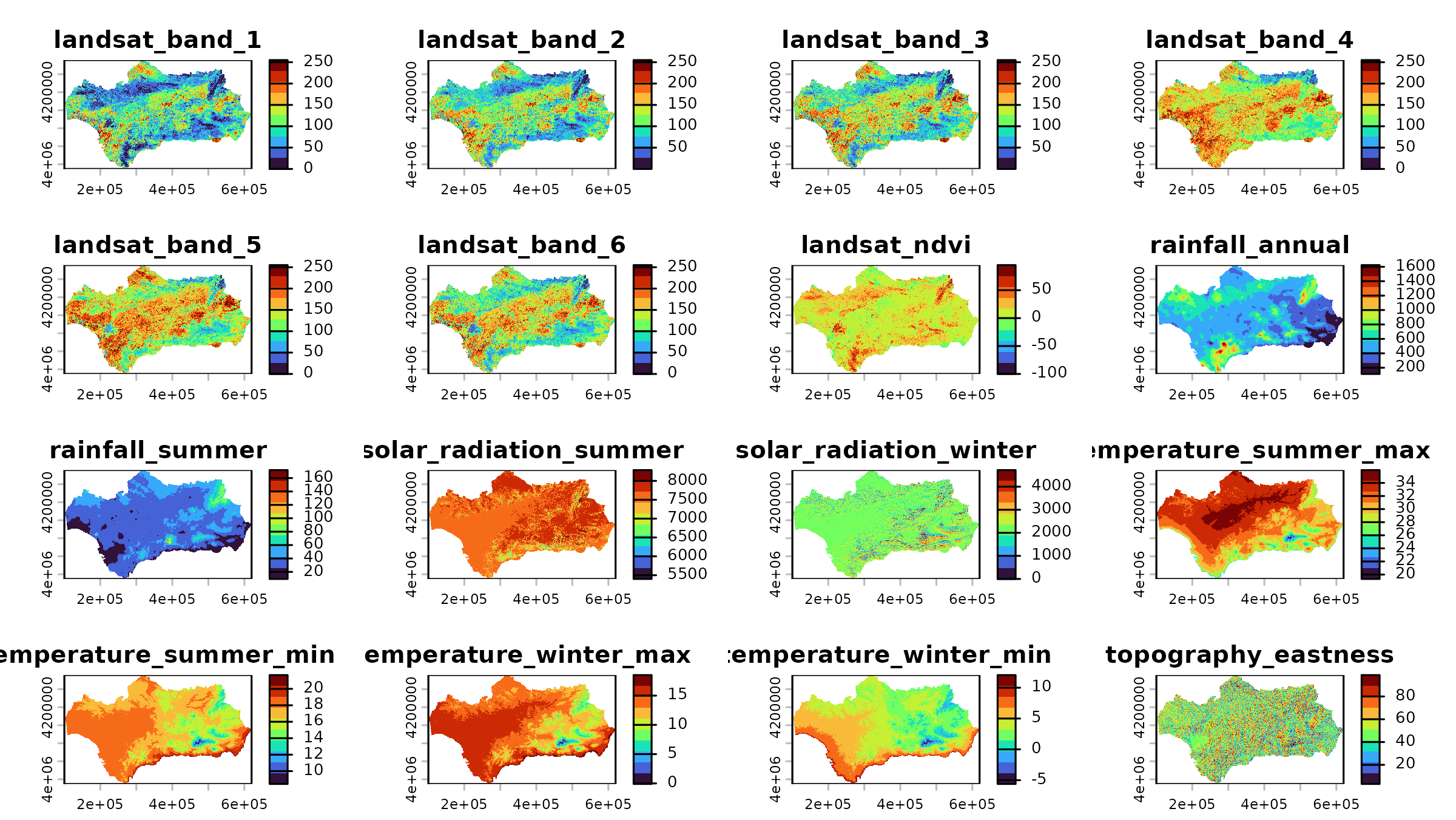
The spatRaster object contains 20 layers, all named in the vector andalusia_predictors.

andalusia_predictors
#>  [1] "landsat_band_1"         "landsat_band_2"         "landsat_band_3"        
#>  [4] "landsat_band_4"         "landsat_band_5"         "landsat_band_6"        
#>  [7] "landsat_ndvi"           "rainfall_annual"        "rainfall_summer"       
#> [10] "solar_radiation_summer" "solar_radiation_winter" "temperature_summer_max"
#> [13] "temperature_summer_min" "temperature_winter_max" "temperature_winter_min"
#> [16] "topography_eastness"    "topography_elevation"   "topography_northness"  
#> [19] "topography_position"    "topography_slope"

Each cell of the raster dataset represents 400 × 400 meters on the ground.

terra::res(andalusia_env)
#> [1] 400 400

We pair each record in andalusia with its corresponding cell values in andalusia_env via terra::extract().

andalusia_env_df <- terra::extract(
  x = andalusia_env,
  y = andalusia,
  ID = FALSE
)

andalusia <- dplyr::bind_cols(
  andalusia,
  andalusia_env_df
) |> 
  na.omit()

dplyr::glimpse(andalusia)
#> Rows: 46,463
#> Columns: 23
#> $ species                <chr> "Quercus_ilex_ballota", "Quercus_ilex_ballota",…
#> $ presence               <int> 1, 1, 1, 1, 1, 1, 1, 1, 1, 1, 1, 1, 1, 1, 1, 1,…
#> $ landsat_band_1         <dbl> 98.85989, 85.23322, 103.63580, 68.93472, 151.53…
#> $ landsat_band_2         <dbl> 102.25950, 91.43609, 97.54510, 65.84269, 159.89…
#> $ landsat_band_3         <dbl> 120.47082, 111.15762, 109.67588, 75.25600, 166.…
#> $ landsat_band_4         <dbl> 133.51358, 139.29692, 97.97874, 65.05608, 166.6…
#> $ landsat_band_5         <dbl> 163.65579, 142.38599, 137.16740, 112.19093, 191…
#> $ landsat_band_6         <dbl> 126.43008, 97.41518, 131.31789, 102.15392, 163.…
#> $ landsat_ndvi           <dbl> 5.58579826, 13.40785694, -6.20389414, -7.286762…
#> $ rainfall_annual        <dbl> 438.1153, 444.4159, 474.9400, 452.7251, 405.607…
#> $ rainfall_summer        <dbl> 43.02710, 44.03641, 43.90874, 44.29456, 41.7911…
#> $ solar_radiation_summer <dbl> 7711.653, 7556.962, 7704.122, 7638.880, 7679.47…
#> $ solar_radiation_winter <dbl> 1951.640, 1325.617, 2056.618, 1669.973, 1830.93…
#> $ temperature_summer_max <dbl> 34.84408, 34.11757, 34.86726, 34.21207, 34.4381…
#> $ temperature_summer_min <dbl> 18.21624, 17.81210, 18.31562, 17.87338, 17.9606…
#> $ temperature_winter_max <dbl> 14.60926, 13.68775, 14.66240, 13.89417, 14.2525…
#> $ temperature_winter_min <dbl> 3.962335, 3.608699, 3.930102, 3.695227, 3.86753…
#> $ topography_eastness    <dbl> 76.10881, 51.90067, 40.87642, 38.99799, 27.1143…
#> $ topography_elevation   <dbl> 347.4608, 454.3534, 356.0224, 455.5842, 404.892…
#> $ topography_northness   <dbl> 68.863571, 86.070404, 73.723236, 68.550499, 60.…
#> $ topography_position    <dbl> -23.6095314, 1.2177124, -46.4343910, -15.821706…
#> $ topography_slope       <dbl> 20.57511139, 10.51053429, 44.49013138, 8.364820…
#> $ geometry               <POINT [m]> POINT (320977.2 4288125), POINT (314577.2…

To speed up code execution in the next section, below we reduce the resolution of andalusia_env by a factor of 4 via aggregation.

andalusia_env <- terra::aggregate(
  x = andalusia_env,
  fact = 4,
  fun = mean
)

terra::res(andalusia_env)
#> [1] 1600 1600

Example Usage

In this section we use the andalusia dataset to build a plant richness model by adding habitat suitability predictions from binary random forest models trained with ranger::ranger().

Before fitting models, we convert presence to a factor (required by ranger for classification modelling) and split the data into two objects: species (presence records) and background. This step will make sense soon!

#convert to factor
andalusia <- dplyr::mutate(
  andalusia,
  presence = factor(presence)
  )

#separate background data
background <- dplyr::filter(
  andalusia,
  species == "background"
  )

#separate species data
presence <- dplyr::filter(
  andalusia,
  species != "background"
  )

Modelling Steps

In this section we define the individual modelling steps for the species Pinus halepensis.

species_name <- "Pinus_halepensis"

First, we filter the records belonging to the target species.

species_presence <- dplyr::filter(
  presence,
  species == species_name
  )

Next, we build a 10 km buffer around the species presences to exclude background points too close to presences. This step helps enhance the contrast between the environmental conditions of presence and background points the model needs to learn from.

species_presence_buffer <- sf::st_buffer(
  x = species_presence,
  dist = 10000 #in meters
) |> 
  sf::st_union()

We use the buffer to identify which background points fall inside of it using sf::st_contains() to remove them.

#identify background points contained by the buffer
background_inside_buffer <- sf::st_contains(
  x = species_presence_buffer,
  y = background,
  sparse = FALSE
) |>
  as.vector()

#select background outside the presence buffer
species_background <- background[!background_inside_buffer, ]

The map below shows the 10 km buffer around the species presences and the background points that remain after filtering.

mapview(
  species_presence, 
  layer.name = "Presence", 
  col.regions = colors[8]
  ) +
mapview(
  species_presence_buffer, 
  col.regions = "gray20", 
  layer.name = "Buffer"
  ) + 
  mapview(
    species_background, 
    col.regions = colors[2], 
    layer.name = "Background"
    )

To finish the data preparation we combine the species presences and the filtered background into a single training data frame, remove the geometry, and select only the response and the predictors

species_training <- dplyr::bind_rows(
  species_presence,
  species_background
) |> 
  sf::st_drop_geometry() |> 
  dplyr::select(
    dplyr::all_of(c("presence", andalusia_predictors))
  )

We train a binary random forest using all predictors, and class weights to account for the imbalance between presences and background records.

The hyperparameters num.trees = 100 and min.node.size = 30 are set below their defaults (500 and 5, respectively) to reduce computation time.

species_model <- ranger::ranger(
  dependent.variable.name = "presence",
  data = species_training,
  case.weights = collinear::case_weights(
    x = species_training$presence
  ),
  num.trees = 100,
  min.node.size = 30
)

At this point we could evaluate this model via spatial cross-validation, assess variable importance, and even check the response curves to understand how it’s working. However, we will skip these steps here to keep the article light of content and computationally efficient.

Below we predict the fitted binary model to every cell of the raster andalusia_env.

species_prediction <- terra::predict(
  object = andalusia_env,
  model = species_model,
  na.rm = TRUE
)

names(species_prediction) <- species_name

The result is a binary raster with values 0 (absence) and 1 (presence). The presence records of the target species are plotted in black.

plot(
  x = species_prediction,
  col = c(colors[2], colors[8])
  )
points(species_presence)

But careful here The values 0 and 1 in the map above do not represent pixel values, they are category labels!

levels(x = species_prediction)[[1]]
#>   value label
#> 1     1     0
#> 2     2     1

To convert the map to numeric with pixel value 0 for label “0” and 1 for label “1” we remove the levels, and subtract 1 to shift pixel values.

#remove levels
levels(x = species_prediction) <- NULL

#shift pixel values
species_prediction <- species_prediction - 1

Now we have the kind of map we need for the next section!

plot(
  x = species_prediction,
  col = c(colors[2], colors[8])
  )

Full Modelling Workflow

In this section we apply the steps learned in the previous section to the 90 plant species in andalusia.

We can start extracting their names to iterate over them.

species_names <- andalusia |>
  dplyr::filter(species != "background") |>
  dplyr::distinct(species) |>
  dplyr::pull(species)

species_names
#>  [1] "Quercus_ilex_ballota"             "Cistus_ladanifer"                
#>  [3] "Quercus_suber"                    "Stipa_tenacissima"               
#>  [5] "Pinus_halepensis"                 "Pistacia_lentiscus"              
#>  [7] "Rosmarinus_officinalis"           "Pinus_pinea"                     
#>  [9] "Olea_europaea_sylvestris"         "Pinus_pinaster"                  
#> [11] "Retama_sphaerocarpa"              "Cistus_salvifolius"              
#> [13] "Cistus_monspeliensis"             "Cistus_albidus"                  
#> [15] "Eucalyptus_globulus"              "Genista_umbellata"               
#> [17] "Pinus_nigra_salzmanii"            "Ulex_parviflorus_parviflorus"    
#> [19] "Anthyllis_cytisoides"             "Rubus_ulmifolius"                
#> [21] "Cistus_populifolius_populifolius" "Festuca_scariosa"                
#> [23] "Calicotome_villosa"               "Calluna_vulgaris"                
#> [25] "Cistus_populifolius_major"        "Juniperus_oxycedrus"             
#> [27] "Erica_arborea"                    "Juniperus_communis"              
#> [29] "Nerium_oleander"                  "Populus_nigra"                   
#> [31] "Ulex_baeticus_baeticus"           "Quercus_faginea"                 
#> [33] "Cytisus_scoparius"                "Arundo_donax"                    
#> [35] "Chamaerops_humilis"               "Castanea_sativa"                 
#> [37] "Arbutus_unedo"                    "Eucalyptus_camaldulensis"        
#> [39] "Populus_alba"                     "Genista_scorpius"                
#> [41] "Olea_europaea_europaea"           "Genista_hirsuta"                 
#> [43] "Cytisus_scoparius_reverchonii"    "Prunus_dulcis"                   
#> [45] "Phragmites_australis"             "Halimium_halimifolium"           
#> [47] "Erinacea_anthyllis"               "Cistus_crispus"                  
#> [49] "Echinospartum_boissieri"          "Thymus_hyemalis"                 
#> [51] "Erica_australis"                  "Artemisia_barrelieri"            
#> [53] "Genista_cinerea"                  "Flueggea_tinctoria"              
#> [55] "Genista_versicolor"               "Salsola_genistoides"             
#> [57] "Quercus_canariensis"              "Genista_florida"                 
#> [59] "Lavandula_lanata"                 "Maytenus_senegalensis_europaea"  
#> [61] "Adenocarpus_decorticans"          "Brachypodium_retusum"            
#> [63] "Ulmus_minor"                      "Genista_speciosa"                
#> [65] "Quercus_pyrenaica"                "Lavandula_stoechas"              
#> [67] "Ceratonia_siliqua"                "Thymbra_capitata"                
#> [69] "Juniperus_phoenicea"              "Thymus_zygis_gracilis"           
#> [71] "Crataegus_monogyna"               "Lavandula_stoechas_sampaiana"    
#> [73] "Phlomis_purpurea"                 "Quercus_fruticosa"               
#> [75] "Tamarix_gallica"                  "Artemisia_campestris_glutinosa"  
#> [77] "Hyparrhenia_hirta"                "Armeria_velutina"                
#> [79] "Securinega_tinctoria"             "Alnus_glutinosa"                 
#> [81] "Hormatophylla_spinosa"            "Erica_andevalensis"              
#> [83] "Loeflingia_baetica"               "Festuca_indigesta"               
#> [85] "Acer_opalus_granatense"           "Sorbus_aria"                     
#> [87] "Acer_monspessulanum"              "Ilex_aquifolium"                 
#> [89] "Prunus_mahaleb"                   "Viola_cazorlensis"

To iterate across these species we wrap our modelling steps in a lapply() call, which will apply the same modelling pipeline to all 90 species. The result is a list of per-species binary rasters, stacked into a single spatRaster with terra::rast().

species_predictions <- lapply(
  X = species_names,
  FUN = function(species_name) {

    species_presence <- presence |>
      dplyr::filter(species == species_name)

    species_presence_buffer <- sf::st_buffer(
      x = species_presence,
      dist = 10000
    ) |>
      sf::st_union()

    background_inside_buffer <- sf::st_contains(
      x = species_presence_buffer,
      y = background,
      sparse = FALSE
    ) |>
      as.vector()

    species_background <- background[!background_inside_buffer, ]

    species_training <- dplyr::bind_rows(
      species_presence,
      species_background
    ) |> 
      sf::st_drop_geometry() |> 
      dplyr::select(
        dplyr::all_of(c("presence", andalusia_predictors))
      )

    species_model <- ranger::ranger(
      dependent.variable.name = "presence",
      data = species_training,
      case.weights = collinear::case_weights(
        x = species_training$presence
      ),
      num.trees = 100,
      min.node.size = 30
    )

    species_prediction <- terra::predict(
      object = andalusia_env,
      model = species_model,
      na.rm = TRUE
    )
    
    levels(x = species_prediction) <- NULL
    
    species_prediction <- species_prediction - 1
    
    names(species_prediction) <- species_name
    
    return(species_prediction)
  }
) |>
  terra::rast()

The resulting multilayer raster contains the individual presence/absence predictions.

plot(
  x = species_predictions,
  col = c(colors[2], colors[8])
  )

Adding these binary predictions together results in a “species richness” raster where each pixel counts how many of the 90 species have predicted suitable habitat at that location.

species_richness <- sum(species_predictions)

Let’s give it a look!

mapview(
  species_richness,
  layer.name = "Plant richness",
  col.regions = colors,
  na.color = "transparent"
)

It looks pretty, doesn’t it?

However, it is important to acknowledge that we took some shortcuts to get there, so we should interpret this “richness” map with care.

That’s all folks, I hope you had as much fun as I did while writing this article!

References

Benito, B.M., Lorite, J., Pérez-Pérez, R., Gómez-Aparicio, L., & Peñas, J. (2014). Forecasting plant range collapse in a mediterranean hotspot: when dispersal uncertainties matter. Diversity and Distributions, 20(1), 72–83. https://doi.org/10.1111/ddi.12148