Linaria nigricans distribution and greenhouse expansion in Andalusia

Overview

The linaria dataset, built from Benito et al. (2009), contains three types of records:

• Species presences (Linaria nigricans occurrence sites)
• Greenhouse presences (competing land-use sites)
• Background points (random samples from the study extent)

Combined with 21 environmental predictors (Landsat reflectance, climate, topography) at 400 m resolution, the dataset is well suited for binary classification, multi-response SDMs, and habitat suitability analysis.

Setup

Data Structure

The dataset is an sf data frame with 7386 rows and 25 columns.

linaria |> 
  head() |> 
  dplyr::glimpse()
#> Rows: 6
#> Columns: 25
#> $ linaria_nigricans      <int> 0, 0, 0, 0, 0, 0
#> $ greenhouses            <int> 1, 1, 1, 1, 1, 1
#> $ landsat_band_1         <dbl> 122.7361, 131.2058, 128.7693, 117.9134, 142.323…
#> $ landsat_band_2         <dbl> 130.0865, 135.1374, 140.4587, 134.2562, 150.022…
#> $ landsat_band_3         <dbl> 135.6665, 138.6600, 151.1233, 147.9056, 156.029…
#> $ landsat_band_4         <dbl> 137.6705, 137.5793, 151.2897, 152.9075, 149.124…
#> $ landsat_band_5         <dbl> 131.5883, 129.5752, 147.2640, 145.7692, 142.580…
#> $ landsat_band_6         <dbl> 128.0193, 129.3456, 143.0903, 141.3965, 138.157…
#> $ landsat_ndvi           <dbl> 0.8935745, -0.2097327, 0.1698296, 2.1492300, -2…
#> $ rainfall_annual        <dbl> 175.6193, 171.8265, 178.8755, 168.6590, 185.399…
#> $ rainfall_summer        <dbl> 25.35585, 24.33438, 26.01632, 22.72672, 26.7352…
#> $ solar_radiation_summer <dbl> 7769.863, 7764.699, 7767.185, 7754.883, 7768.42…
#> $ solar_radiation_winter <dbl> 2414.235, 2398.743, 2409.010, 2391.854, 2436.68…
#> $ temperature_summer_max <dbl> 31.19968, 31.27113, 31.29720, 31.31935, 31.3081…
#> $ temperature_summer_min <dbl> 17.88333, 17.97116, 17.92983, 18.10378, 17.9232…
#> $ temperature_winter_max <dbl> 14.32534, 14.44624, 14.40007, 14.62476, 14.3911…
#> $ temperature_winter_min <dbl> 5.040048, 5.155740, 5.103079, 5.360068, 5.15614…
#> $ topography_eastness    <dbl> 33.27220, 33.43419, 33.64509, 44.18529, 41.8191…
#> $ topography_elevation   <dbl> 457.2828, 432.8701, 441.4741, 398.9463, 442.908…
#> $ topography_northness   <dbl> 17.243651, 16.443365, 15.332311, 13.336531, 7.8…
#> $ topography_position    <dbl> 0.5508171, 0.8273488, -4.5827132, -0.4132942, 2…
#> $ topography_slope       <dbl> 2.989993, 2.701621, 2.819398, 2.356359, 2.77472…
#> $ x                      <dbl> 597188.7, 597508.7, 596268.7, 598608.7, 595028.…
#> $ y                      <dbl> 4147393, 4146933, 4146733, 4146353, 4146013, 41…
#> $ geometry               <POINT [m]> POINT (597188.7 4147393), POINT (597508.7 41469…

It has two binary response variables (see linaria_responses):

linaria_responses
#> [1] "linaria_nigricans" "greenhouses"

Both response variables encode binary outcomes: 1 for confirmed presence, 0 for all other record types.

The map below shows all three record types by colour.

linaria_mapped <- linaria |>
  dplyr::mutate(
    record_type = dplyr::case_when(
      linaria_nigricans == 1L ~ "Linaria nigricans",
      greenhouses == 1L      ~ "Greenhouse",
      TRUE                   ~ "Background"
    )
  )

mapview::mapview(
  linaria_mapped,
  zcol = "record_type",
  layer.name = "Record type",
  col.regions = c("gray60", "darkgreen", "violet")
)

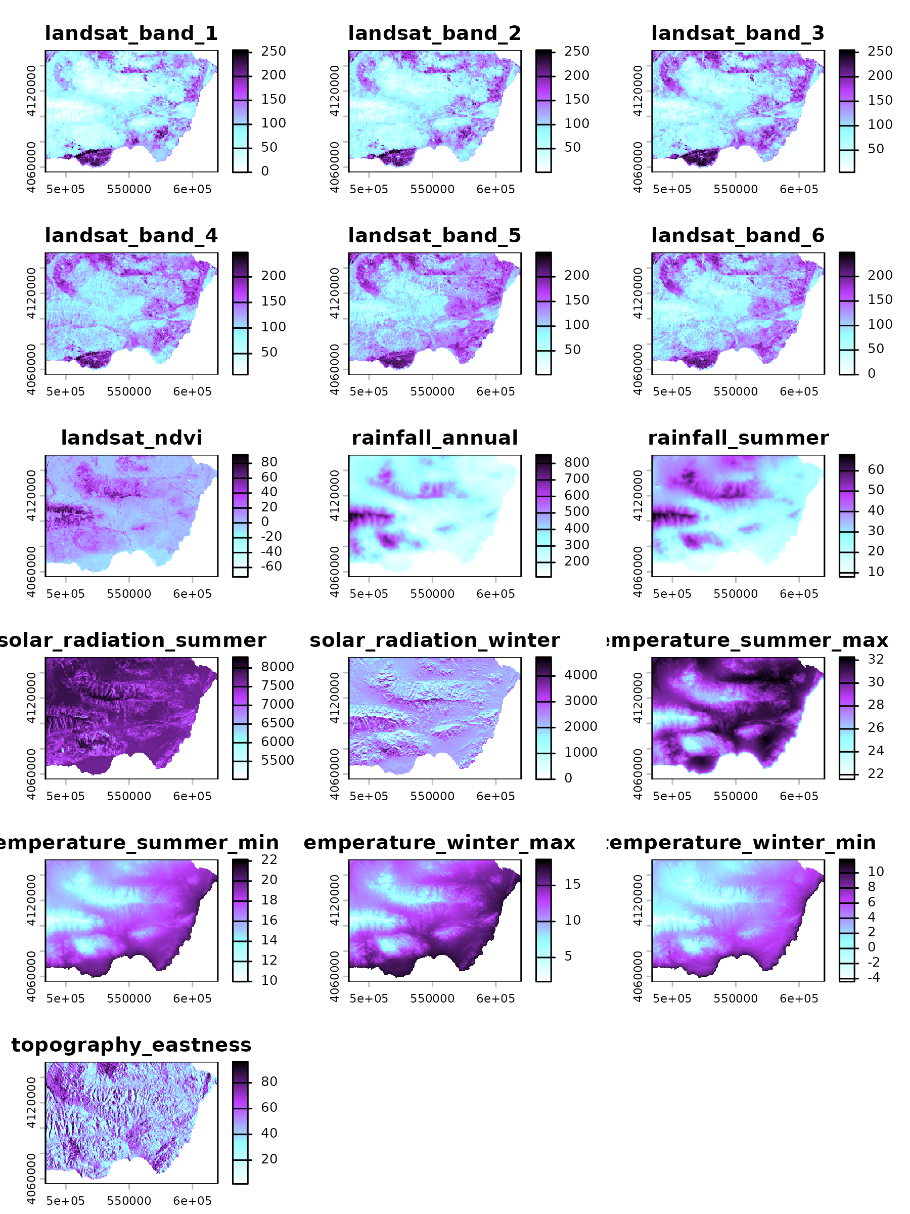
The dataset includes 20 remote sensing, topographic, and climate predictors.

linaria_predictors
#>  [1] "landsat_band_1"         "landsat_band_2"         "landsat_band_3"        
#>  [4] "landsat_band_4"         "landsat_band_5"         "landsat_band_6"        
#>  [7] "landsat_ndvi"           "rainfall_annual"        "rainfall_summer"       
#> [10] "solar_radiation_summer" "solar_radiation_winter" "temperature_summer_max"
#> [13] "temperature_summer_min" "temperature_winter_max" "temperature_winter_min"
#> [16] "topography_eastness"    "topography_elevation"   "topography_northness"  
#> [19] "topography_position"    "topography_slope"

Example Usage

Greenhouse agriculture and Linaria nigricans compete for the same lowland territory in eastern Andalusia. Following an approach similar to Benito et al. (2009), we fit two separate habitat suitability models using maxnet, one for L. nigricans and one for greenhouses, predict them across the study region, and combine them into an extinction-risk surface by multiplying the two suitability layers and rescaling to 0–100.

Environmental raster

The environmental raster (same extent, 400 m resolution, EPSG:25830) is loaded with linaria_extra(). When the vignette renders, the raster file linaria_env.tif is read from disk without re-downloading.

linaria_env <- spatialData::linaria_extra()

plot(linaria_env)

Fitting SDMs with maxnet

Each maxnet() call treats rows where the response equals 1 as presences and all other rows (including the opposite response’s presences and background points) as background. This pseudo-absence design lets us model each response against the full environmental backdrop of the study region.

training_df <- sf::st_drop_geometry(linaria)

linaria_model <- maxnet::maxnet(
  p = training_df[["linaria_nigricans"]],
  data = training_df[, linaria_predictors]
)

greenhouses_model <- maxnet::maxnet(
  p = training_df[["greenhouses"]],
  data = training_df[, linaria_predictors]
)

We project each model onto the environmental raster using terra::predict() with type = "cloglog", which returns values bounded between 0 and 1 that can be interpreted as occurrence probability. The option clamp = TRUE restricts predictions to the environmental envelope seen during training.

linaria_prediction <- terra::predict(
  object = linaria_env,
  model  = linaria_model,
  type   = "cloglog",
  clamp  = TRUE,
  na.rm  = TRUE
)
names(linaria_prediction) <- "linaria"

greenhouses_prediction <- terra::predict(
  object = linaria_env,
  model  = greenhouses_model,
  type   = "cloglog",
  clamp  = TRUE,
  na.rm  = TRUE
)
names(greenhouses_prediction) <- "greenhouses"

plot(
  linaria_prediction,
  col  = viridis::turbo(100),
  main = "Linaria nigricans suitability"
)

plot(
  greenhouses_prediction,
  col  = viridis::turbo(100),
  main = "Greenhouse suitability"
)

Extinction-risk composite

The relative extinction-risk surface is the product of the two suitability layers. Areas with high scores represent places where L. nigricans is likely to occur and where greenhouses are likely to expand, indicating high-risk zones.

linaria_risk <- terra::stretch(
  x = linaria_prediction * greenhouses_prediction, 
  minv = 0, 
  maxv = 100
  )

mapview(
  linaria_risk,
  col.regions  = viridis::turbo(100),
  layer.name = "Relative risk (0–100)"
) + 
  mapview(
    linaria |> 
      dplyr::filter(
        linaria_nigricans == 1
      ),
    layer.name = "Linaria presence",
    alpha.regions = 0
  )

The original data is from 2008. Notice how several presence records in the high-risk areas are already covered by greenhouses.

Conclusion

The linaria dataset provides a compact but ecologically rich testbed for multi-response binary classification: one response captures species habitat suitability, the other captures the spatial footprint of the main threatening land use. This structure is ideal for comparative SDM workflows, land-use conflict analyses, or any task requiring simultaneous modelling of species and threat distributions.

The extinction-risk analysis above shows how combining two MaxEnt predictions into a spatially explicit composite can pinpoint the areas where conservation action is most urgent — the approach introduced by Benito et al. (2009) for Linaria nigricans in Andalusia.

References

Benito, B.M., Martínez-Ortega, M.M., Munoz, L.M., Lorite, J. & Penas, J. (2009). Assessing extinction-risk of endangered plants using species distribution models: a case study of habitat depletion caused by the spread of greenhouses. Biodiversity and Conservation, 18(9), 2509–2520. https://doi.org/10.1007/s10531-009-9604-8
Peñas, J., Benito, B., Lorite, J., et al. (2011). Habitat fragmentation in arid zones: a case study of Linaria nigricans under land use changes (SE Spain). Environmental Management, 48, 168–176. https://doi.org/10.1007/s00267-011-9663-y
Benito, B.P.d., Peñas, J.G.d. (2008). Greenhouses, land use change, and predictive models: MaxEnt and Geomod working together. In: Paegelow, M., Olmedo, M.T.C. (eds) Modelling Environmental Dynamics. Environmental Science and Engineering. Springer, Berlin, Heidelberg. https://doi.org/10.1007/978-3-540-68498-5_11