Overview
The neanderthal dataset contains records of Neanderthal
archaeological sites from Marine Isotope Stage 5e (Last Interglacial,
~130,000-115,000 years ago), combined with 25 paleoclimate and
topographic predictor variables. This dataset was built to support
binary classification, species distribution modelling, and habitat
suitability analysis.
Setup
The code below loads the R libraries and example data required to run this tutorial.
library(dplyr)
library(sf)
library(mapview)
library(terra)
library(mgcv)
library(plotmo)
library(collinear)
library(spatialData)

data(
  neanderthal,
  neanderthal_response,
  neanderthal_predictors,
  package = "spatialData"
)

#colors for environmental variables and uncertainty layer
env_colors <- grDevices::hcl.colors(
  palette = "YlGnBu",
  n = 10
)

#colors for neanderthal suitability
neanderthal_colors <- grDevices::hcl.colors(
  palette = "Zissou 1",
  n = 10
)

#colors for presences and background records
neanderthal_color <- neanderthal_colors[10]
background_color <- neanderthal_colors[1]

neanderthal <- dplyr::mutate(
  neanderthal,
  color = ifelse(
    test = presence == 1,
    yes = neanderthal_color,
    no = background_color
  )
)
Data Structure
The dataset is an sf POINT dataframe (EPSG 4326) with
227 rows and 28 columns, and no missing data.
dplyr::glimpse(neanderthal)
#> Rows: 227
#> Columns: 28
#> $ presence             <int> 1, 1, 1, 1, 1, 1, 1, 1, 1, 1, 1, 1, 1, 1, 1, 1, 1…
#> $ bio1                 <dbl> 93.90861, 101.39613, 98.43701, 80.31912, 67.72340…
#> $ bio10                <dbl> 230.8535, 193.2386, 196.0572, 208.2075, 193.7100,…
#> $ bio11                <dbl> -40.628402, 19.409437, 7.986982, -47.536219, -58.…
#> $ bio12                <dbl> 1016.7842, 634.9449, 651.3601, 481.9939, 598.3581…
#> $ bio13                <dbl> 124.79270, 86.20893, 78.12757, 64.77663, 79.24467…
#> $ bio14                <dbl> 42.9601370, 20.1204209, 23.6468781, 17.5191646, 2…
#> $ bio15                <dbl> 28.78959, 34.29474, 27.51153, 40.68027, 36.12821,…
#> $ bio16                <dbl> 321.4307, 235.2489, 220.1406, 189.4942, 228.7584,…
#> $ bio17                <dbl> 141.42826, 103.49764, 107.45727, 59.94072, 84.456…
#> $ bio18                <dbl> 306.99387, 125.23646, 155.59023, 179.19781, 213.6…
#> $ bio19                <dbl> 174.55667, 150.36287, 140.85947, 60.03907, 84.465…
#> $ bio2                 <dbl> 107.35804, 80.55478, 86.42271, 101.75828, 100.366…
#> $ bio3                 <dbl> 24.97327, 29.14201, 29.00000, 24.82866, 24.62171,…
#> $ bio4                 <dbl> 10434.941, 6795.361, 7319.844, 9877.545, 9766.644…
#> $ bio5                 <dbl> 315.4290, 259.6066, 268.1590, 290.8134, 275.5202,…
#> $ bio6                 <dbl> -109.914922, -12.303463, -26.610513, -115.376691,…
#> $ bio7                 <dbl> 425.3439, 271.9101, 294.7695, 406.1901, 401.8273,…
#> $ bio8                 <dbl> 219.387741, 95.264316, 89.376189, 200.248222, 186…
#> $ bio9                 <dbl> -23.84609, 52.21129, 49.78763, -41.15274, -58.285…
#> $ topo_aspect          <dbl> 203.37818, 149.00686, 169.84060, 142.45523, 149.4…
#> $ topo_diversity_local <dbl> 7.1118334, 6.2437519, 1.2860197, -3.1426907, -0.7…
#> $ topo_diversity       <dbl> 78.13295, 74.73658, 73.03239, 67.50587, 71.77473,…
#> $ topo_elev            <dbl> 240.97322, 62.10563, 32.56124, 110.95158, 348.351…
#> $ topo_slope           <dbl> 2.0600362, 0.9570366, 0.3261872, 1.3632851, 1.354…
#> $ topo_wetness         <dbl> -3.142004, -3.236383, -1.925804, -3.006190, -4.24…
#> $ geometry             <POINT [°]> POINT (15.8632 46.1654), POINT (1.8785 50.1…
#> $ color                <chr> "#F5191C", "#F5191C", "#F5191C", "#F5191C", "#F51…
The response variable is presence (see
neanderthal_response), a integer binary variable indicating
Neanderthal presence (1) or pseudo-absence (0).
table(neanderthal$presence)
#>
#>   0   1
#> 178  49
The locations of the presence and background records are mapped below.
mapview::mapview(
  neanderthal |>
    dplyr::mutate(
      presence = as.factor(presence)
    ),
  zcol = "presence",
  layer.name = "Presence",
  col.regions = neanderthal$color
)
The dataset includes 25 palaeoclimatic (last interglacial) and topographic predictors.
neanderthal_predictors
#> [1] "bio1" "bio10" "bio11"
#> [4] "bio12" "bio13" "bio14"
#> [7] "bio15" "bio16" "bio17"
#> [10] "bio18" "bio19" "bio2"
#> [13] "bio3" "bio4" "bio5"
#> [16] "bio6" "bio7" "bio8"
#> [19] "bio9" "topo_aspect" "topo_diversity_local"
#> [22] "topo_diversity" "topo_elev" "topo_slope"
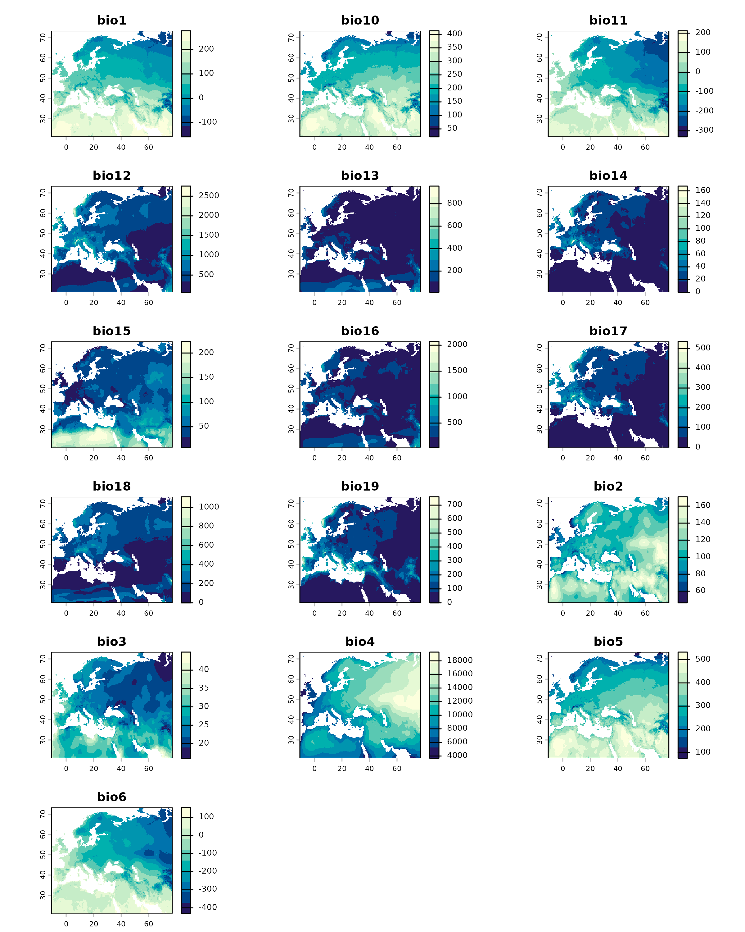
#> [25] "topo_wetness"There is a companion raster dataset loaded via
neanderthal_extra().
neanderthal_env <- spatialData::neanderthal_extra()

plot(
  x = neanderthal_env,
  nc = 3,
  col = env_colors,
  )
Example Usage
In this section we use neanderthal to model habitat
suitability via an ensemble of univariate GAMs, one per predictor.
The neanderthal data has 49 presences. Fitting a model
with all predictors at once might lead to overparameterization and
overfitting. To avoid this potential issue, we will fit univariate GAM
models between presence and each environmental predictor. Each model in
the ensemble follows this structure:
m <- mgcv::gam(
  formula = presence ~ s(
    bio1,
    k = ceiling(sum(neanderthal$presence)/10)
    ),
  data = sf::st_drop_geometry(neanderthal),
  family = stats::quasibinomial(link = "logit"),
  weights = collinear::case_weights(
    x = neanderthal$presence
    ),
  select = TRUE
)mgcv::gam(): GAM models replace the linear terms used in GLMs with smoothing splines that better represent non-linear relationships between presence and environment.s(..., k = ceiling(sum(neanderthal$presence)/10): smoothing splines capture non-linear relationships between presence and each predictor. The basis dimensionkis set relative to the number of presences, keeping the smooth complexity well within the data budget.quasibinomial(link = "logit"): handles the overdispersion introduced by pseudo-absences and the fractional case weights, which a standardbinomialfamily would reject.weights = case_weights(...): inverse-frequency weights ensure that presences and pseudo-absences contribute equally to model fit regardless of their imbalance.
sample_weights <- collinear::case_weights(x = neanderthal$presence)
table(sample_weights)
#> sample_weights
#> 0.00280898876404494  0.0102040816326531
#> 178 49-
select = TRUE: adds a shrinkage penalty so that uninformative smooths can be penalized to zero, acting as automatic term selection.
After all relevant models are fitted, we will ensemble their predictions using their intrinsic AUC (probability of giving a higher suitability to a presence than to a background point) as weights.
collinear::score_auc(
  o = neanderthal$presence,
  p = stats::predict(m, type = "response")
)
#> [1] 0.8357028
Multicollinearity Filtering
There are many redundant predictors in neanderthal. To
mitigate this issue, here we apply collinear::collinear()
to select a non-redundant subset of the most relevant predictors. The
function ranks all predictors by the AUC of univariate binomial GAM
models with case weights (very similar to the ones we’ll use for the
habitat suitability model!), and then applies a multicollinearity
filtering that preserves the most important ones.
neanderthal_selection <- collinear::collinear(
  df = neanderthal,
  responses = neanderthal_response,
  predictors = neanderthal_predictors,
  f = collinear::f_binomial_gam
)
#>
#> collinear::collinear()
#> └── collinear::validate_arg_df()
#>     └── collinear::drop_geometry_column(): dropping geometry column from 'df'.
#>
#> collinear::collinear(): setting 'max_cor' to 0.517.
#>
#> collinear::collinear(): setting 'max_vif' to 2.8923.
#>
#> collinear::collinear(): selected predictors:
#>  - bio17
#>  - bio1
#>  - bio7
#>  - bio8
#>  - topo_slope
#>  - bio13
#>  - topo_diversity
#>  - topo_wetness
#>  - topo_aspect
The names of the selected predictors are in the vector below.
neanderthal_selection$presence$selection
#> [1] "bio17"          "bio1"           "bio7"           "bio8"
#> [5] "topo_slope"     "bio13"          "topo_diversity" "topo_wetness"
#> [9] "topo_aspect"
#> attr(,"validated")
#> [1] TRUE
Model Fitting
The code below fits the univariate GAM models. Notice that models with an intrinsic AUC below 0.75 are ignored.
neanderthal_models <- lapply(
  X = neanderthal_selection$presence$selection,
  FUN = \(x) {

    model_formula <- as.formula(
        paste0(
          "presence ~ s(",
          x,
          ", k = ",
          ceiling(sum(neanderthal$presence) / 10),
          ")"
        )
      )

    model <- mgcv::gam(
      formula = model_formula,
      data = sf::st_drop_geometry(neanderthal),
      family = stats::quasibinomial(link = "logit"),
      weights = collinear::case_weights(
        x = neanderthal$presence
      ),
      select = TRUE
    )

    auc <- collinear::score_auc(
      o = neanderthal$presence,
      p = stats::predict(
        object = model,
        type = "response"
        )
      )

    model$auc <- auc

    model

  }
)

names(neanderthal_models) <- neanderthal_selection$presence$selection
Let’s take a look at the performance of these univariate models.
neanderthal_auc <- lapply(
  X = neanderthal_models,
  FUN = \(x) x$auc
) |>
  unlist()

neanderthal_auc
#>          bio17           bio1           bio7           bio8     topo_slope
#>      0.8225178      0.8357028      0.8049759      0.7455859      0.7984407
#>          bio13 topo_diversity   topo_wetness    topo_aspect
#>      0.7860582      0.7043109      0.6113277      0.6315065
Several of these models have very low intrinsic AUC scores, meaning that they lack the ability to discriminate properly between presences and background points. We are going to ignore all models with an AUC below 0.75.
#keep models with AUC >= 0.75
neanderthal_auc <- neanderthal_auc[neanderthal_auc >= 0.75]
#remove bad models from the models list
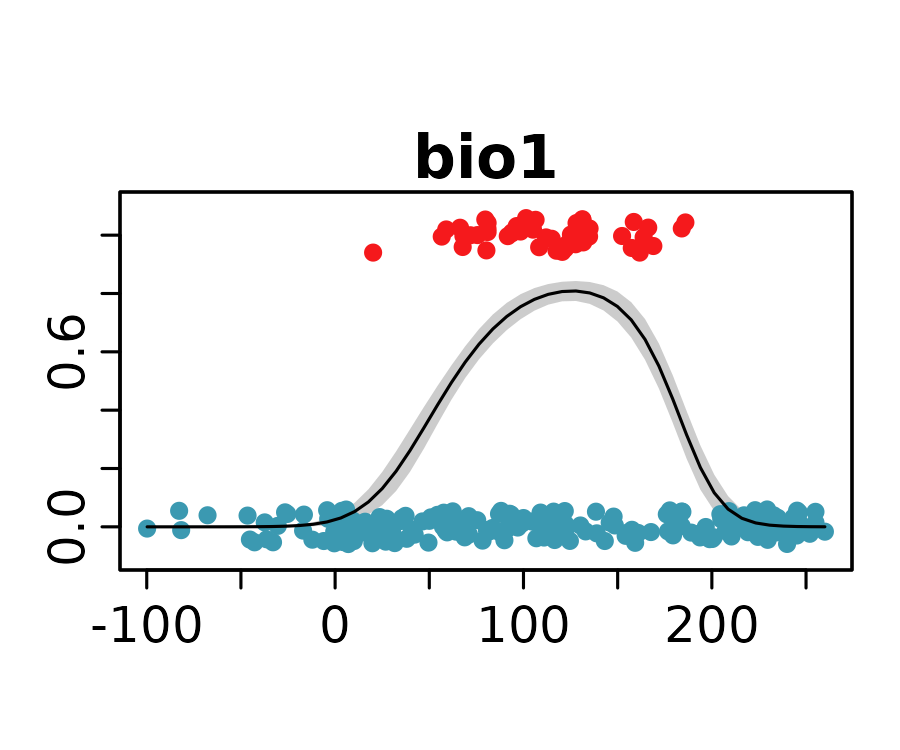
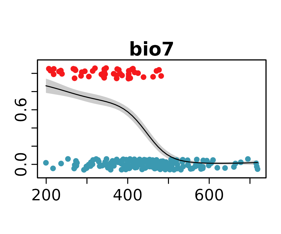
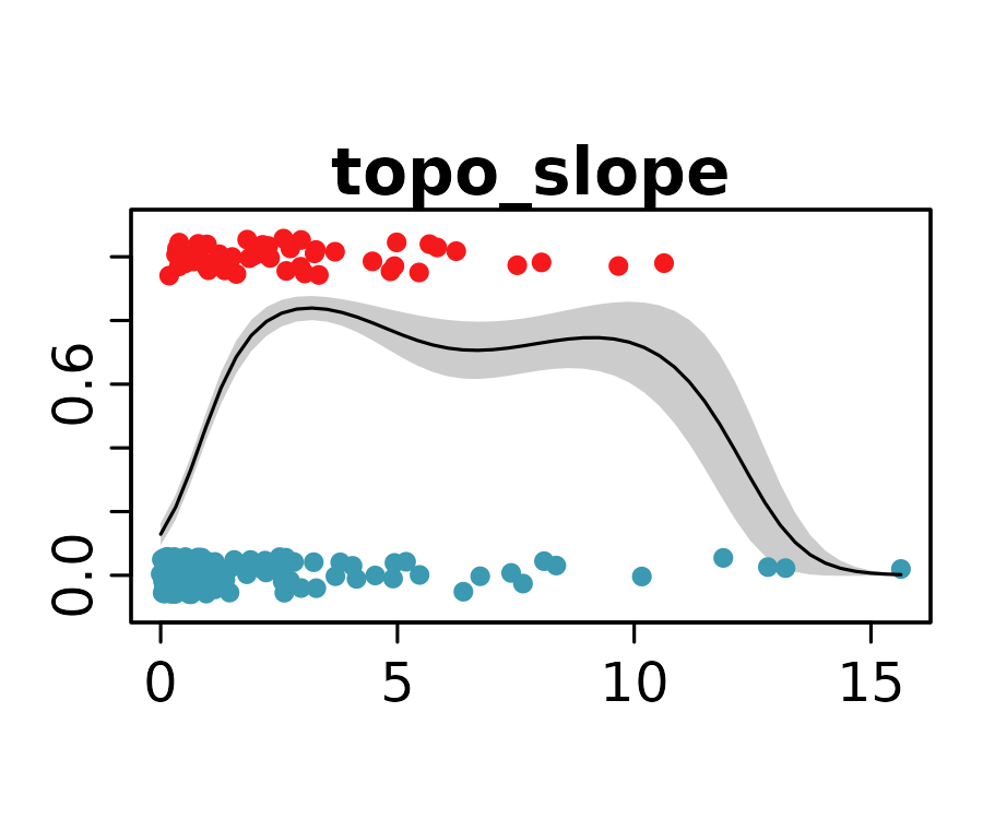
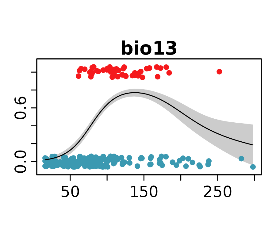
neanderthal_models <- neanderthal_models[names(neanderthal_auc)]The response curves below show the predicted probability of Neanderthal presence for the selected univariate models.
lapply(
  X = names(neanderthal_models),
  FUN = \(x) {
  x <- plotmo::plotmo(
    object = neanderthal_models[[x]],
    type = "response",
    level = 0.95,
    level.shade = "gray80",
    main = x,
    caption = "",
    pt.col = neanderthal$color,
    jitter = 0.3,
    smooth.col = 0
  )
}) |>
  invisible()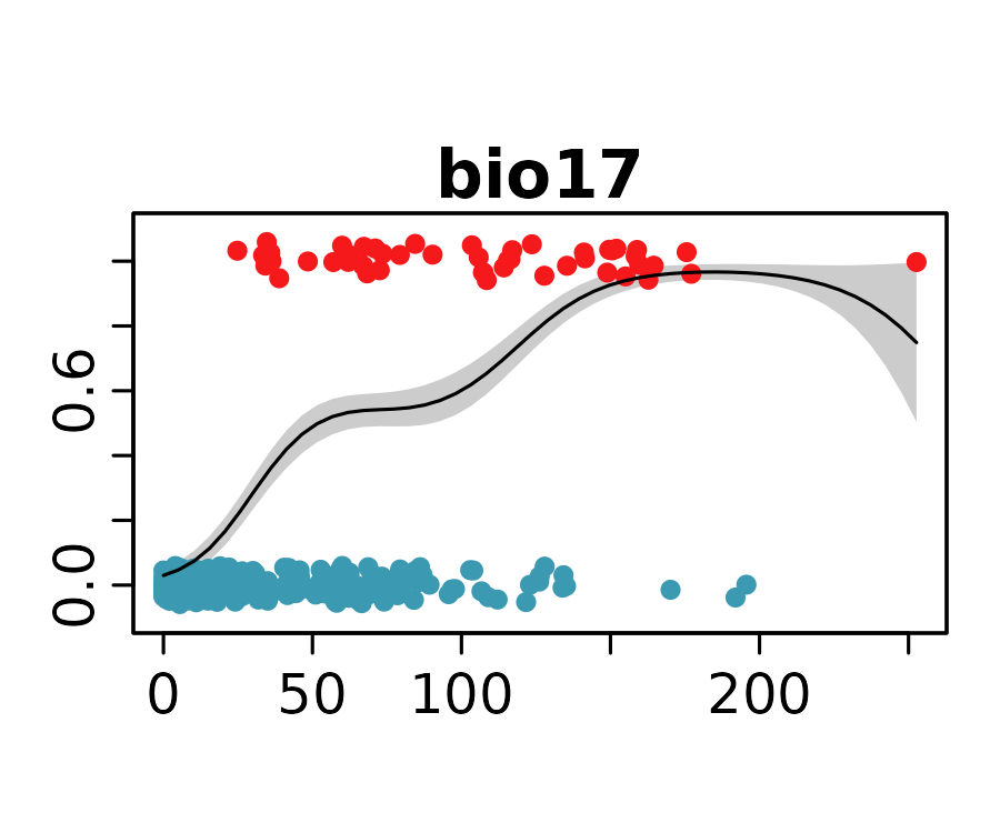
Habitat Suitability Map
To build the weighted ensemble of univariate models we first need to
predict each univariate model over the spatRaster object
neanderthal_env.
neanderthal_predictions <- lapply(
  X = names(neanderthal_models),
  FUN = \(x) {
    terra::predict(
      object = neanderthal_env,
      model = neanderthal_models[[x]],
      type = "response",
      na.rm = TRUE
    )
  }
) |>
  terra::rast()

names(neanderthal_predictions) <- names(neanderthal_models)
The resulting object is a spatRaster where each layer
represents a univariate suitability map.
plot(
  x = neanderthal_predictions,
  col = neanderthal_colors
  )
To build the ensemble, we apply terra::weighted.mean()
to the individual model predictions and their intrinsic AUCs.
neanderthal_suitability <- terra::weighted.mean(
x = neanderthal_predictions,
w = neanderthal_auc
)
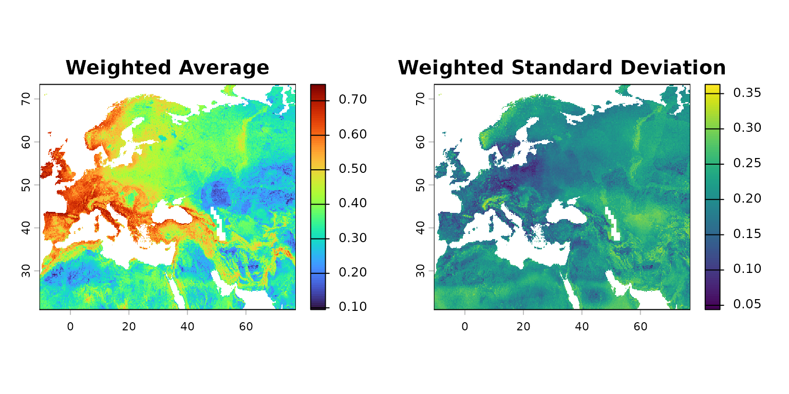
names(neanderthal_suitability) <- "suitability"The map below shows the high-suitability values in warmer colors.
mapview(
  x = neanderthal_suitability,
  layer.name = "Suitability",
  col.regions = neanderthal_colors,
  na.color = "transparent"
)
To finish, we can
#extract predicted values for all records
neanderthal$prediction <- terra::extract(
    x = neanderthal_suitability,
    y = neanderthal,
    ID = FALSE
  ) |>
    dplyr::pull(
      suitability
    )

#remove NA data (not supported by score_auc())
neanderthal <- na.omit(neanderthal)

#compute intrinsic AUC
collinear::score_auc(
  o = neanderthal$presence,
  p = neanderthal$prediction
)
#> [1] 0.9091353
That’s good to see: the AUC of the ensemble is better than any AUC of the univariate models, which is the whole point of building this kind of ensemble modelling.
Conclusion
The ensemble of univariate GAMs, weighted by cross-validated AUC, provides a robust picture of Neanderthal habitat suitability during the Last Interglacial.
References
Benito, B.M., et al. (2017). The ecological niche and distribution of Neanderthals during the Last Interglacial. Journal of Biogeography, 44, 51–61. https://doi.org/10.1111/jbi.12845
Nielsen, T.K., Benito, B.M., Svenning, J.-C., Sandel, B., McKerracher, L., Riede, F., & Kjærgaard, P.C. (2017). Investigating Neanderthal dispersal above 55°N in Europe during the Last Interglacial Complex. Quaternary International, 431, 88–103. https://doi.org/10.1016/j.quaint.2015.10.039